In-class Exercise 2: Geospatial Data Wrangling with R

Published

January 20, 2023

Modified

January 31, 2023

Installing the R packages

First, we need to check if we have the three R packages to be used for the In-Class Excercise (sf ,tidyverse and funModelling) installed. If not, we need to install it automatically. The below code checks if the packages are already installed, else it will install the packages for us. However, before running the below code, ensure that 'packman' package has been installed in your RStudio.

pacman::p_load(sf, tidyverse, funModeling)

Importing the Geospatial Dataset

The geoBoundaries Dataset

To Import the Geospatial data, run the following code. Ensure that the directory of the files and the file name is correct. By running the code, the data will be in meters and it will be in simple feature format.

geoNGA <- st_read("data/geospatial", 
                  layer = "geoBoundaries-NGA-ADM2") %>%
  st_transform(crs = 26392)

Reading layer `geoBoundaries-NGA-ADM2' from data source 
  `/Users/shambhavigoenka/Desktop/School/Geo/IS415-GAA/in-class_ex/in-class_ex02/data/geospatial' 
  using driver `ESRI Shapefile'
Simple feature collection with 774 features and 5 fields
Geometry type: MULTIPOLYGON
Dimension:     XY
Bounding box:  xmin: 2.668534 ymin: 4.273007 xmax: 14.67882 ymax: 13.89442
Geodetic CRS:  WGS 84

Importing the NGA Dataset

To Import the NGAdata, run the following code. Ensure that the directory of the files and the file name is correct.

NGA <- st_read("data/geospatial", 
                  layer = "nga_admbnda_adm2_osgof_20190417") %>%
  st_transform(crs = 26392)

Reading layer `nga_admbnda_adm2_osgof_20190417' from data source 
  `/Users/shambhavigoenka/Desktop/School/Geo/IS415-GAA/in-class_ex/in-class_ex02/data/geospatial' 
  using driver `ESRI Shapefile'
Simple feature collection with 774 features and 16 fields
Geometry type: MULTIPOLYGON
Dimension:     XY
Bounding box:  xmin: 2.668534 ymin: 4.273007 xmax: 14.67882 ymax: 13.89442
Geodetic CRS:  WGS 84

Importing Aspatial data

Similar to the Geospatial data, import the Aspatial data, however, remember that the data is in CSV format and hence, read_csv() must be used

wp_nga <- read_csv("data/aspatial/WPdx.csv") %>%
  filter(`#clean_country_name` == "Nigeria")

Converting Aspatial Data into Geospatial

We now convert the newly extracted Aspatial data (wp_nga) into point sf dataframe using the below code.

wp_nga$Geometry = st_as_sfc(wp_nga$`New Georeferenced Column`)
wp_nga

# A tibble: 97,478 × 75
   row_id `#source`      #lat_…¹ #lon_…² #repo…³ #stat…⁴ #wate…⁵ #wate…⁶ #wate…⁷
    <dbl> <chr>            <dbl>   <dbl> <chr>   <chr>   <chr>   <chr>   <chr>  
 1 158721 Federal Minis…    5.07    6.62 02/19/… Yes     Boreho… Well    Mechan…
 2 158892 Federal Minis…    5.09    7.09 02/06/… Yes     Boreho… Well    Hand P…
 3 323117 Federal Minis…    5.91    8.77 08/31/… Yes     Boreho… Well    Hand P…
 4 300176 Federal Minis…    5.23    7.32 05/17/… Yes     Boreho… Well    Mechan…
 5 324346 Federal Minis…    6.88    3.36 08/17/… Yes     Boreho… Well    Mechan…
 6 297273 Federal Minis…    6.59    3.29 05/26/… Yes     Boreho… Well    Mechan…
 7 296853 Federal Minis…    6.60    3.26 06/02/… Yes     Boreho… Well    Mechan…
 8 323866 Federal Minis…    6.20    6.73 09/18/… Yes     Boreho… Well    Mechan…
 9 297044 Federal Minis…    6.61    3.30 05/26/… Yes     Boreho… Well    Mechan…
10 324321 Federal Minis…    6.96    3.60 08/16/… Yes     Boreho… Well    Mechan…
# … with 97,468 more rows, 66 more variables: `#water_tech_category` <chr>,
#   `#facility_type` <chr>, `#clean_country_name` <chr>, `#clean_adm1` <chr>,
#   `#clean_adm2` <chr>, `#clean_adm3` <chr>, `#clean_adm4` <chr>,
#   `#install_year` <dbl>, `#installer` <chr>, `#rehab_year` <lgl>,
#   `#rehabilitator` <lgl>, `#management_clean` <chr>, `#status_clean` <chr>,
#   `#pay` <chr>, `#fecal_coliform_presence` <chr>,
#   `#fecal_coliform_value` <dbl>, `#subjective_quality` <chr>, …

wp_sf <- st_sf(wp_nga, crs=4326)
wp_sf

Simple feature collection with 97478 features and 74 fields
Geometry type: POINT
Dimension:     XY
Bounding box:  xmin: 2.707441 ymin: 4.301812 xmax: 14.21828 ymax: 13.86568
Geodetic CRS:  WGS 84
# A tibble: 97,478 × 75
   row_id `#source`      #lat_…¹ #lon_…² #repo…³ #stat…⁴ #wate…⁵ #wate…⁶ #wate…⁷
 *  <dbl> <chr>            <dbl>   <dbl> <chr>   <chr>   <chr>   <chr>   <chr>  
 1 158721 Federal Minis…    5.07    6.62 02/19/… Yes     Boreho… Well    Mechan…
 2 158892 Federal Minis…    5.09    7.09 02/06/… Yes     Boreho… Well    Hand P…
 3 323117 Federal Minis…    5.91    8.77 08/31/… Yes     Boreho… Well    Hand P…
 4 300176 Federal Minis…    5.23    7.32 05/17/… Yes     Boreho… Well    Mechan…
 5 324346 Federal Minis…    6.88    3.36 08/17/… Yes     Boreho… Well    Mechan…
 6 297273 Federal Minis…    6.59    3.29 05/26/… Yes     Boreho… Well    Mechan…
 7 296853 Federal Minis…    6.60    3.26 06/02/… Yes     Boreho… Well    Mechan…
 8 323866 Federal Minis…    6.20    6.73 09/18/… Yes     Boreho… Well    Mechan…
 9 297044 Federal Minis…    6.61    3.30 05/26/… Yes     Boreho… Well    Mechan…
10 324321 Federal Minis…    6.96    3.60 08/16/… Yes     Boreho… Well    Mechan…
# … with 97,468 more rows, 66 more variables: `#water_tech_category` <chr>,
#   `#facility_type` <chr>, `#clean_country_name` <chr>, `#clean_adm1` <chr>,
#   `#clean_adm2` <chr>, `#clean_adm3` <chr>, `#clean_adm4` <chr>,
#   `#install_year` <dbl>, `#installer` <chr>, `#rehab_year` <lgl>,
#   `#rehabilitator` <lgl>, `#management_clean` <chr>, `#status_clean` <chr>,
#   `#pay` <chr>, `#fecal_coliform_presence` <chr>,
#   `#fecal_coliform_value` <dbl>, `#subjective_quality` <chr>, …

Project Transformation

We now transform the projection from wgs84 to appropriate projected coordinate system of Nigeria.

wp_sf <- wp_sf %>%
  st_transform(crs = 26392)

Geospatial Data Cleaning

Excluding redundent fields

NGA <- NGA %>%
  select(c(3:4,8:9))

Checking for duplicate name

It is important to check for duplicate name in the data main data fields. Using duplicate(), we can flag out the LGA names.

NGA$ADM2_EN[duplicated(NGA$ADM2_EN)==TRUE]

[1] "Bassa"    "Ifelodun" "Irepodun" "Nasarawa" "Obi"      "Surulere"

The printout above shows that there are 6 LGAs with the same name,. A Google search using the coordinates showed that there are LGAs with the same name but are located in different states.

NGA$ADM2_EN[94] <- "Bassa, Kogi"
NGA$ADM2_EN[95] <- "Bassa, Plateau"
NGA$ADM2_EN[304] <- "Ifelodun, Kwara"
NGA$ADM2_EN[305] <- "Ifelodun, Osun"
NGA$ADM2_EN[355] <- "Irepodun, Kwara"
NGA$ADM2_EN[356] <- "Irepodun, Osun"
NGA$ADM2_EN[519] <- "Nasarawa, Kano"
NGA$ADM2_EN[520] <- "Nasarawa, Nasarawa"
NGA$ADM2_EN[546] <- "Obi, Benue"
NGA$ADM2_EN[547] <- "Obi, Nasarawa"
NGA$ADM2_EN[693] <- "Surulere, Lagos"
NGA$ADM2_EN[694] <- "Surulere, Oyo"

Check if there are any duplicated codes now

NGA$ADM2_EN[duplicated(NGA$ADM2_EN)==TRUE]

character(0)

Data Wrangling for Water Point Data

freq(data = wp_sf,
     input = '#status_clean')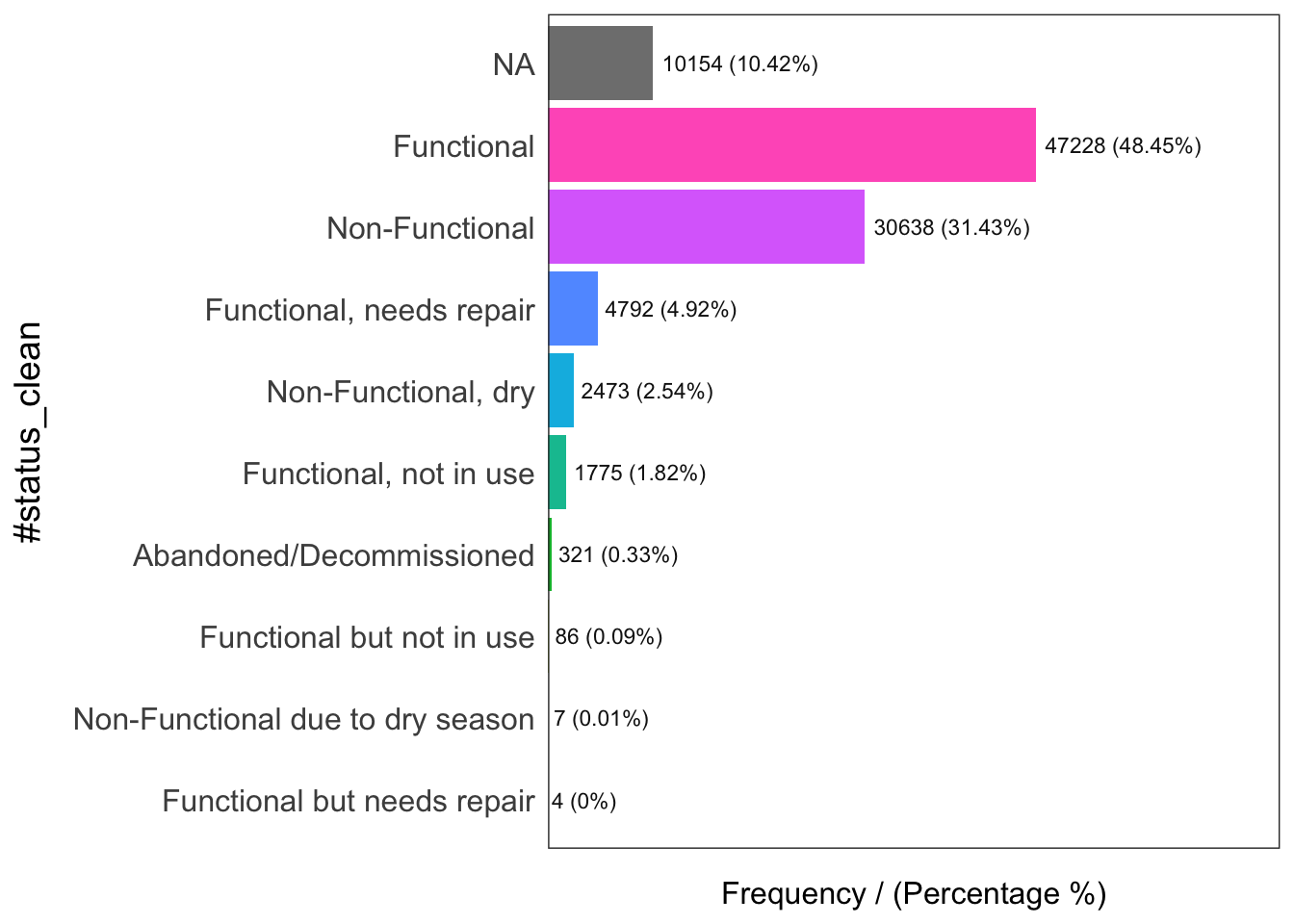

                      #status_clean frequency percentage cumulative_perc
1                        Functional     47228      48.45           48.45
2                    Non-Functional     30638      31.43           79.88
3                              <NA>     10154      10.42           90.30
4          Functional, needs repair      4792       4.92           95.22
5               Non-Functional, dry      2473       2.54           97.76
6            Functional, not in use      1775       1.82           99.58
7          Abandoned/Decommissioned       321       0.33           99.91
8         Functional but not in use        86       0.09          100.00
9  Non-Functional due to dry season         7       0.01          100.01
10      Functional but needs repair         4       0.00          100.00

wp_sf_nga <- wp_sf %>%
  rename(status_clean = '#status_clean') %>%
  select(status_clean) %>%
  mutate(status_clean = replace_na(
    status_clean, "unknown"))

Extracting Water Point Data

wp_functional <- wp_sf_nga %>%
  filter(status_clean %in%
           c("Functional",
             "Functional but not in use",
             "Functional but needs repair"))

wp_nonfunctional <- wp_sf_nga %>%
  filter(status_clean %in%
           c("Abandoned/Decommissioned",
             "Abandoned",
             "Non-Functional due to dry season",
             "Non-Functional",
             "Non functional due to dry season"))

wp_unknown <- wp_sf_nga %>%
  filter(status_clean == "unknown")

Next, the code chunk below is used to perform a quick EDA on the derived sf data.frames.

freq(data = wp_functional,
     input = 'status_clean')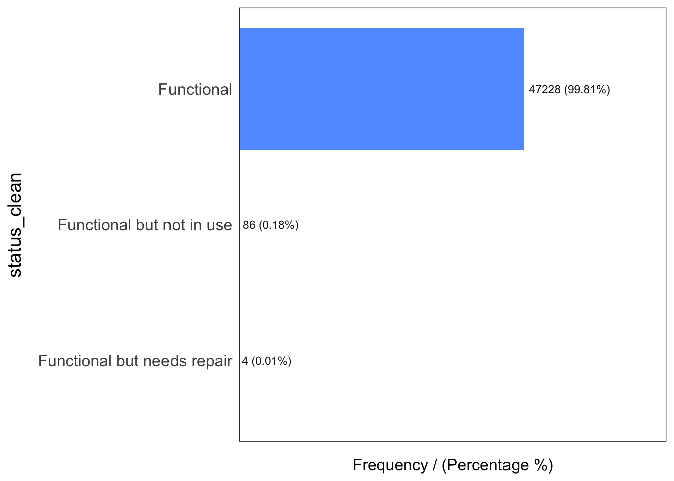

                 status_clean frequency percentage cumulative_perc
1                  Functional     47228      99.81           99.81
2   Functional but not in use        86       0.18           99.99
3 Functional but needs repair         4       0.01          100.00

freq(data = wp_nonfunctional,
     input = 'status_clean')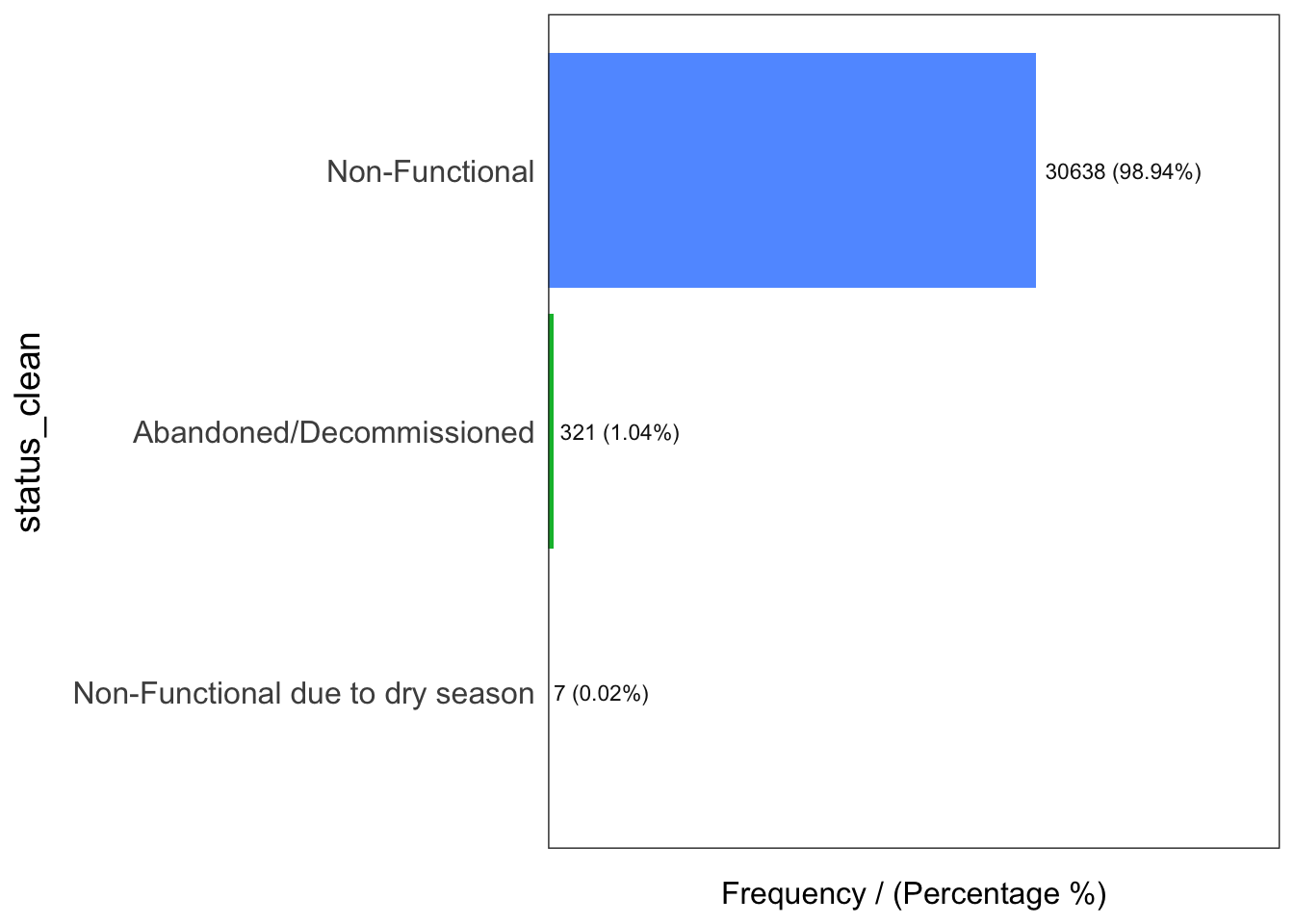

                      status_clean frequency percentage cumulative_perc
1                   Non-Functional     30638      98.94           98.94
2         Abandoned/Decommissioned       321       1.04           99.98
3 Non-Functional due to dry season         7       0.02          100.00

freq(data = wp_unknown,
     input = 'status_clean')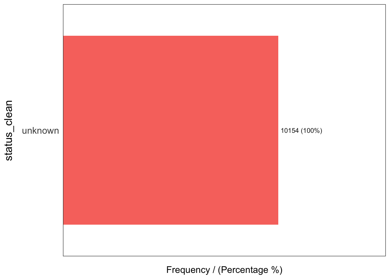

  status_clean frequency percentage cumulative_perc
1      unknown     10154        100             100

Performing Point-in Polygon Count

NGA_wp <- NGA %>%
  mutate(`total_wp` = lengths(
    st_intersects(NGA, wp_sf_nga))) %>%
  mutate(`wp_functional` = lengths(
    st_intersects(NGA, wp_functional))) %>%
  mutate(`wp_nonfunctional` = lengths(
    st_intersects(NGA, wp_nonfunctional))) %>%
  mutate(`wp_unknown` = lengths(
    st_intersects(NGA, wp_unknown)))

Visualising attributes by using statistical graphs

ggplot(data= NGA_wp,
       aes(x = total_wp)) + 
  geom_histogram(bins = 20,
                 color="black",
                 fill="light blue") + 
  geom_vline(aes(xintercept=mean(
    total_wp, na.rm=T)),
              color="red",
              linetype="dashed",
              size=0.8) + 
  ggtitle("Distribution of total water points by LGA") + 
  xlab("No. of water points") + 
  ylab("No. of\nLGAs") + 
  theme(axis.title.y = element_text(angle = 0))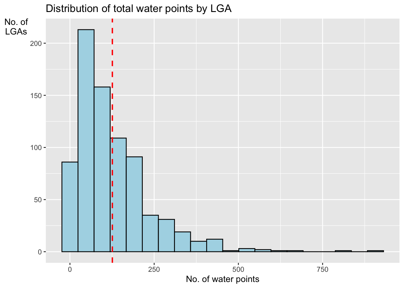

Saving the Analytical data in rds format

write_rds(NGA_wp, "data/rds/NGA_wp.rds")