In-Class Exercise 6: Choropleth Mapping

1.0 Overview

2.0 Setup

2.1 Installing and Loading the R Packages

pacman::p_load(sf, tmap, sfdep, tidyverse)
#keep tidyverse at the end for dependency checking

2.2 The Data

• Hunan, a geospatial data set in ESRI shapefile format, and

• Hunan_2012, an attribute data set in csv format.

2.2.1 Import Geospatial Data

hunan <- st_read(dsn = "data/geospatial", 
                 layer = "Hunan")

Reading layer `Hunan' from data source 
  `/Users/shambhavigoenka/Desktop/School/Geo/IS415-GAA/in-class_ex/in-class_ex06/data/geospatial' 
  using driver `ESRI Shapefile'
Simple feature collection with 88 features and 7 fields
Geometry type: POLYGON
Dimension:     XY
Bounding box:  xmin: 108.7831 ymin: 24.6342 xmax: 114.2544 ymax: 30.12812
Geodetic CRS:  WGS 84

2.2.2 Import attribute table

hunan2012 <- read_csv("data/aspatial/Hunan_2012.csv")

2.2.3 Combine both data frames using left join

In order to retain the geospatial properties, the left data frame must be the sf data.frame(i.e. hunan)

hunan_GDPPC <- left_join(hunan,hunan2012)%>%
  select(1:4, 7, 15) #name, id, name, engtype, 7 - county, 15 - gdppc

2.2.3 Choropleth Map

tmap_mode("plot")
tm_shape(hunan_GDPPC) + 
  tm_fill("GDPPC",
          style = "quantile",
          palette = "Blues",
          title = "GDPPC") + 
  tm_layout(main.title = "Distribution of GDP per capita by district, Hunan Province",
            main.title.position = "center",
            main.title.size = 1.2,
            legend.height = 0.45,
            legend.width = 0.35,
            frame = TRUE) + 
  tm_borders(alpha = 0.5) + 
  # tm_text("NAME_3", size=0.5) + 
  tm_compass(type = "8star", size = 2) + 
  tm_scale_bar() + #decimal degree projection turns into km using great circle calculation 
  tm_grid(alpha = 0.2)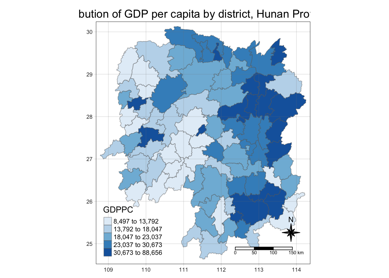

3.0 Identify area neighbors

3.1 Contiguity Spatial Weights

Redundant in later steps = 4.1

3.1.1 Derive neighbor’s list using Queen’s method

# -- st version
nb_queen <- hunan_GDPPC %>%
  mutate(nb = st_contiguity(geometry), #default is queen
         .before = 1) #place as first column

#wm_q <- poly2nd(hunan_GDPPC, queen = TRUE) -- sp version

3.1.2 Derive neighbor’s list using Rook’s method

nb_rook <- hunan_GDPPC %>%
  mutate(nb = st_contiguity(geometry), #default is queen
         queen = FALSE,
         .before = 1) #place as first column

3.1.3 Identifying higher order neighbors

Queen Method

nb2_queen <-  hunan_GDPPC %>% 
  mutate(nb = st_contiguity(geometry),
         nb2 = st_nb_lag_cumul(nb, 2),
         .before = 1)

4.0 K-nearest neighbors method

4.1 Contiguity Spatial Weights

4.1.1 Derive neighbor’s list using Queen’s method

wm_q <- hunan_GDPPC %>%
  mutate(nb = st_contiguity(geometry),
         wt = st_weights(nb,
                         style = "W"),
         .before = 1) 

4.1.2 Derive neighbor’s list using Rook’s method

wm_r <- hunan %>%
  mutate(nb = st_contiguity(geometry,
                            queen = FALSE),
         wt = st_weights(nb),
         .before = 1) 

5.0 Distance-based Weights

5.1 Distance band method

Fixed distance criterion - lower = 0, upper = whatever

geo <- sf::st_geometry(hunan_GDPPC)
nb <- st_knn(geo, longlat = TRUE)
dists <- unlist(st_nb_dists(geo, nb))

summary(dists)

   Min. 1st Qu.  Median    Mean 3rd Qu.    Max. 
  21.56   29.11   36.89   37.34   43.21   65.80 

Maximum nearest neighbor distance is 65.80km so threshold of 66km means there will be at least one neighbor

wm_fd <- hunan_GDPPC %>%
  mutate(nb = st_dist_band(geometry,
                           upper = 66),
               wt = st_weights(nb),
               .before = 1)

5.2 Adaptive Distance Method

wm_ad <- hunan_GDPPC %>% 
  mutate(nb = st_knn(geometry,
                     k=8),
         wt = st_weights(nb),
               .before = 1)

5.3 Inverse Distance Method

wm_idw <- hunan_GDPPC %>%
  mutate(nb = st_contiguity(geometry),
         wts = st_inverse_distance(nb, geometry,
                                   scale = 1,
                                   alpha = 1),
         .before = 1)