pacman::p_load(sf, maptools, raster, spatstat, tmap, kableExtra, tidyverse, funModeling, sfdep)Take Home Exercise 1
1.0 Overview
1.1 Background
This analysis aims to apply appropriate spatial point patterns analysis methods to discover the geographical distribution of functional and non-function water points and their co-locations if any in Osun State, Nigeria.
1.2 Task
Exploratory Spatial Data Analysis (ESDA)
Second-order Spatial Point Pattern Analysis
Spatial Correlation Analysis
2.0 Setup
2.1 Import Packages
sf - Used for handling geospatial data
tidyVerse - Used for data transformation and presentation
tmap, maptools, kableExtra - Used for visualizing dataframes and plots
spatstat - Used for point-pattern analysis
sfdep - Used for functions not in spdep
raster - Used to handle gridded spatial data
3.0 Data Wrangling
3.1 Datasets Used
Code
# initialise a dataframe of our geospatial and aspatial dataset details
datasets <- data.frame(
Type=c("Geospatial",
"Geospatial",
"Geospatial",
"Geospatial",
"Geospatial",
"Geospatial",
"Geospatial",
"Geospatial",
"Geospatial",
"Geospatial",
"Geospatial",
"Geospatial",
"Geospatial",
"Geospatial",
"Aspatial"),
Name=c("geoBoundaries-NGA-ADM2",
"geoBoundaries-NGA-ADM2",
"geoBoundaries-NGA-ADM2",
"geoBoundaries-NGA-ADM2",
"geoBoundaries-NGA-ADM2",
"geoBoundaries-NGA-ADM2",
"nga_admbnda_adm2_osgof_20190417",
"nga_admbnda_adm2_osgof_20190417",
"nga_admbnda_adm2_osgof_20190417",
"nga_admbnda_adm2_osgof_20190417",
"nga_admbnda_adm2_osgof_20190417",
"nga_admbnda_adm2_osgof_20190417",
"nga_admbnda_adm2_osgof_20190417",
"nga_admbnda_adm2_osgof_20190417",
"WPdx"),
Format=c(".dbf",
".geojson",
".prj",
".shp",
".shx",
".topojson",
".CPG",
".dbf",
".prj",
".sbn",
".sbx",
".shp",
".shp",
".shx",
".csv"),
Source=c("[geoBoundaries](https://www.geoboundaries.org/index.html#getdata)",
"[geoBoundaries](https://www.geoboundaries.org/index.html#getdata)",
"[geoBoundaries](https://www.geoboundaries.org/index.html#getdata)",
"[geoBoundaries](https://www.geoboundaries.org/index.html#getdata)",
"[geoBoundaries](https://www.geoboundaries.org/index.html#getdata)",
"[geoBoundaries](https://www.geoboundaries.org/index.html#getdata)",
"[Humanitarian Data Exchange](https://data.humdata.org/dataset/cod-ab-nga)",
"[Humanitarian Data Exchange](https://data.humdata.org/dataset/cod-ab-nga)",
"[Humanitarian Data Exchange](https://data.humdata.org/dataset/cod-ab-nga)",
"[Humanitarian Data Exchange](https://data.humdata.org/dataset/cod-ab-nga)",
"[Humanitarian Data Exchange](https://data.humdata.org/dataset/cod-ab-nga)",
"[Humanitarian Data Exchange](https://data.humdata.org/dataset/cod-ab-nga)",
"[Humanitarian Data Exchange](https://data.humdata.org/dataset/cod-ab-nga)",
"[Humanitarian Data Exchange](https://data.humdata.org/dataset/cod-ab-nga)",
"[ WPdx Global Data Repositories](https://www.waterpointdata.org/access-data/)")
)
# with reference to this guide on kableExtra:
# https://cran.r-project.org/web/packages/kableExtra/vignettes/awesome_table_in_html.html
# kable_material is the name of the kable theme
# 'hover' for to highlight row when hovering, 'scale_down' to adjust table to fit page width
library(knitr)
library(kableExtra)
kable(datasets, caption="Datasets Used") %>%
kable_material("hover", latex_options="scale_down")| Type | Name | Format | Source |
|---|---|---|---|
| Geospatial | geoBoundaries-NGA-ADM2 | .dbf | [geoBoundaries](https://www.geoboundaries.org/index.html#getdata) |
| Geospatial | geoBoundaries-NGA-ADM2 | .geojson | [geoBoundaries](https://www.geoboundaries.org/index.html#getdata) |
| Geospatial | geoBoundaries-NGA-ADM2 | .prj | [geoBoundaries](https://www.geoboundaries.org/index.html#getdata) |
| Geospatial | geoBoundaries-NGA-ADM2 | .shp | [geoBoundaries](https://www.geoboundaries.org/index.html#getdata) |
| Geospatial | geoBoundaries-NGA-ADM2 | .shx | [geoBoundaries](https://www.geoboundaries.org/index.html#getdata) |
| Geospatial | geoBoundaries-NGA-ADM2 | .topojson | [geoBoundaries](https://www.geoboundaries.org/index.html#getdata) |
| Geospatial | nga_admbnda_adm2_osgof_20190417 | .CPG | [Humanitarian Data Exchange](https://data.humdata.org/dataset/cod-ab-nga) |
| Geospatial | nga_admbnda_adm2_osgof_20190417 | .dbf | [Humanitarian Data Exchange](https://data.humdata.org/dataset/cod-ab-nga) |
| Geospatial | nga_admbnda_adm2_osgof_20190417 | .prj | [Humanitarian Data Exchange](https://data.humdata.org/dataset/cod-ab-nga) |
| Geospatial | nga_admbnda_adm2_osgof_20190417 | .sbn | [Humanitarian Data Exchange](https://data.humdata.org/dataset/cod-ab-nga) |
| Geospatial | nga_admbnda_adm2_osgof_20190417 | .sbx | [Humanitarian Data Exchange](https://data.humdata.org/dataset/cod-ab-nga) |
| Geospatial | nga_admbnda_adm2_osgof_20190417 | .shp | [Humanitarian Data Exchange](https://data.humdata.org/dataset/cod-ab-nga) |
| Geospatial | nga_admbnda_adm2_osgof_20190417 | .shp | [Humanitarian Data Exchange](https://data.humdata.org/dataset/cod-ab-nga) |
| Geospatial | nga_admbnda_adm2_osgof_20190417 | .shx | [Humanitarian Data Exchange](https://data.humdata.org/dataset/cod-ab-nga) |
| Aspatial | WPdx | .csv | [ WPdx Global Data Repositories](https://www.waterpointdata.org/access-data/) |
3.2 Geospatial Data
3.2.1 Load Data
Import Geospatial data and filter out Osun State. Transform WGS 48 coordinate system to projected coordinate system with Nigeria’s ESPG - 26293
osun <- st_read(dsn = "data/geospatial/",
layer = "nga_admbnda_adm2_osgof_20190417") %>%
filter(ADM1_EN == "Osun") %>%
st_transform(crs = 26392)Reading layer `nga_admbnda_adm2_osgof_20190417' from data source
`/Users/shambhavigoenka/Desktop/School/Geo/IS415-GAA/take_home_ex/take_home_ex01/data/geospatial'
using driver `ESRI Shapefile'
Simple feature collection with 774 features and 16 fields
Geometry type: MULTIPOLYGON
Dimension: XY
Bounding box: xmin: 2.668534 ymin: 4.273007 xmax: 14.67882 ymax: 13.89442
Geodetic CRS: WGS 84glimpse(osun)Rows: 30
Columns: 17
$ Shape_Leng <dbl> 1.7951405, 0.7101503, 0.9199564, 0.8502782, 0.5212768, 0.60…
$ Shape_Area <dbl> 0.062436080, 0.024818478, 0.038002894, 0.030445804, 0.01221…
$ ADM2_EN <chr> "Aiyedade", "Aiyedire", "Atakumosa East", "Atakumosa West",…
$ ADM2_PCODE <chr> "NG030001", "NG030002", "NG030003", "NG030004", "NG030005",…
$ ADM2_REF <chr> "Aiyedade", "Aiyedire", "Atakumosa East", "Atakumosa West",…
$ ADM2ALT1EN <chr> NA, NA, NA, NA, NA, NA, NA, NA, NA, NA, NA, NA, NA, NA, NA,…
$ ADM2ALT2EN <chr> NA, NA, NA, NA, NA, NA, NA, NA, NA, NA, NA, NA, NA, NA, NA,…
$ ADM1_EN <chr> "Osun", "Osun", "Osun", "Osun", "Osun", "Osun", "Osun", "Os…
$ ADM1_PCODE <chr> "NG030", "NG030", "NG030", "NG030", "NG030", "NG030", "NG03…
$ ADM0_EN <chr> "Nigeria", "Nigeria", "Nigeria", "Nigeria", "Nigeria", "Nig…
$ ADM0_PCODE <chr> "NG", "NG", "NG", "NG", "NG", "NG", "NG", "NG", "NG", "NG",…
$ date <date> 2016-11-29, 2016-11-29, 2016-11-29, 2016-11-29, 2016-11-29…
$ validOn <date> 2019-04-17, 2019-04-17, 2019-04-17, 2019-04-17, 2019-04-17…
$ validTo <date> NA, NA, NA, NA, NA, NA, NA, NA, NA, NA, NA, NA, NA, NA, NA…
$ SD_EN <chr> "Osun West", "Osun West", "Osun East", "Osun East", "Osun C…
$ SD_PCODE <chr> "NG03003", "NG03003", "NG03002", "NG03002", "NG03001", "NG0…
$ geometry <MULTIPOLYGON [m]> MULTIPOLYGON (((213526.6 34..., MULTIPOLYGON (…3.2.2 Data Preprocessing
3.2.2.1 Exclude redundant fields
osun <- osun %>%
select(c(3:4, 8:9))3.2.2.2 Invalid Geometries
length(which(st_is_valid(osun) == FALSE))[1] 0Everything is valid
3.2.2.3 Checking for Duplicate Names
osun$ADM2_EN[duplicated(osun$ADM2_EN)==TRUE]character(0)No duplicate Local Government Areas (LGAs)
3.2.2.4 Remove Missing Values
osun[rowSums(is.na(osun))!=0,]Simple feature collection with 0 features and 4 fields
Bounding box: xmin: NA ymin: NA xmax: NA ymax: NA
Projected CRS: Minna / Nigeria Mid Belt
[1] ADM2_EN ADM2_PCODE ADM1_EN ADM1_PCODE geometry
<0 rows> (or 0-length row.names)3.2.3 Initial Visualisation
plot(st_geometry(osun), main="Osun State")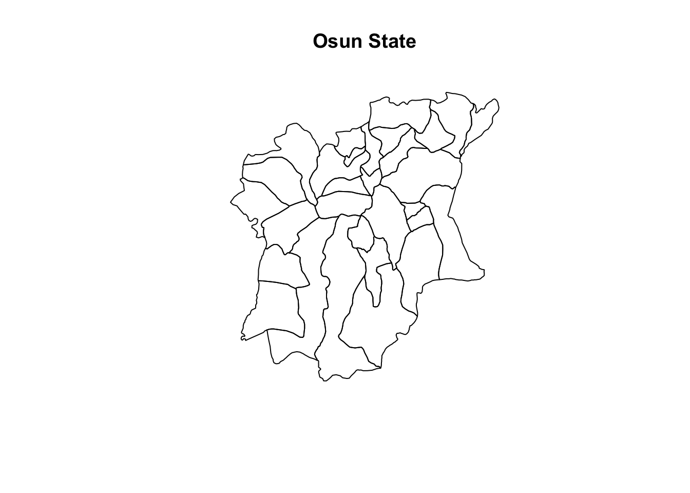
3.3 Aspatial Data
3.3.1 Load Data
Import Aspatial data and filter out Osun State.
wp <- read_csv("data/aspatial/WPdx.csv") %>%
filter(`#clean_country_name` == "Nigeria" & `#clean_adm1` == "Osun")glimpse(wp)Rows: 5,557
Columns: 70
$ row_id <dbl> 429123, 70566, 70578, 66401, 422190, 422…
$ `#source` <chr> "GRID3", "Federal Ministry of Water Reso…
$ `#lat_deg` <dbl> 8.020000, 7.317741, 7.759448, 8.031187, …
$ `#lon_deg` <dbl> 5.060000, 4.785507, 4.563998, 4.637400, …
$ `#report_date` <chr> "08/29/2018 12:00:00 AM", "05/11/2015 12…
$ `#status_id` <chr> "Unknown", "No", "No", "No", "Unknown", …
$ `#water_source_clean` <chr> NA, "Protected Shallow Well", "Borehole"…
$ `#water_source_category` <chr> NA, "Well", "Well", "Well", NA, NA, "Wel…
$ `#water_tech_clean` <chr> "Tapstand", "Mechanized Pump", "Mechaniz…
$ `#water_tech_category` <chr> "Tapstand", "Mechanized Pump", "Mechaniz…
$ `#facility_type` <chr> "Improved", "Improved", "Improved", "Imp…
$ `#clean_country_name` <chr> "Nigeria", "Nigeria", "Nigeria", "Nigeri…
$ `#clean_adm1` <chr> "Osun", "Osun", "Osun", "Osun", "Osun", …
$ `#clean_adm2` <chr> "Ifedayo", "Atakumosa East", "Osogbo", "…
$ `#clean_adm3` <chr> NA, NA, NA, NA, NA, NA, NA, NA, NA, NA, …
$ `#clean_adm4` <chr> NA, NA, NA, NA, NA, NA, NA, NA, NA, NA, …
$ `#install_year` <dbl> NA, NA, NA, 2004, NA, NA, 2006, 2014, 20…
$ `#installer` <chr> NA, NA, NA, NA, NA, NA, NA, NA, NA, NA, …
$ `#rehab_year` <lgl> NA, NA, NA, NA, NA, NA, NA, NA, NA, NA, …
$ `#rehabilitator` <lgl> NA, NA, NA, NA, NA, NA, NA, NA, NA, NA, …
$ `#management_clean` <chr> NA, NA, NA, NA, NA, NA, NA, NA, NA, "Com…
$ `#status_clean` <chr> NA, "Abandoned/Decommissioned", "Abandon…
$ `#pay` <chr> NA, "No", "No", "No", NA, NA, "No", "No"…
$ `#fecal_coliform_presence` <chr> NA, NA, NA, NA, NA, NA, NA, NA, NA, NA, …
$ `#fecal_coliform_value` <dbl> NA, NA, NA, NA, NA, NA, NA, NA, NA, NA, …
$ `#subjective_quality` <chr> NA, "Acceptable quality", "Acceptable qu…
$ `#activity_id` <chr> "6054e946-2573-45bf-ab7c-0ddaa68a61b4", …
$ `#scheme_id` <chr> NA, NA, NA, NA, NA, NA, NA, NA, NA, NA, …
$ `#wpdx_id` <chr> "6FW723C6+222", "6FV68Q9P+36R", "6FV6QH5…
$ `#notes` <chr> "Rt Hon Kola Oluwawole Water Tap", "Temi…
$ `#orig_lnk` <chr> "https://nigeria.africageoportal.com/dat…
$ `#photo_lnk` <chr> NA, "https://akvoflow-55.s3.amazonaws.co…
$ `#country_id` <chr> "NG", "NG", "NG", "NG", "NG", "NG", "NG"…
$ `#data_lnk` <chr> "https://catalog.waterpointdata.org/data…
$ `#distance_to_primary_road` <dbl> 4474.22234, 10130.42742, 167.82235, 4133…
$ `#distance_to_secondary_road` <dbl> 1883.98780, 17466.35720, 838.91849, 1162…
$ `#distance_to_tertiary_road` <dbl> 1885.874322, 2376.832183, 1181.107236, 9…
$ `#distance_to_city` <dbl> 40100.268, 31549.222, 2449.293, 16704.19…
$ `#distance_to_town` <dbl> 8120.871, 24652.907, 9463.295, 5176.899,…
$ water_point_history <chr> "{\"2018-08-29\": {\"source\": \"GRID3\"…
$ rehab_priority <dbl> NA, NA, NA, NA, NA, NA, NA, NA, NA, NA, …
$ water_point_population <dbl> NA, NA, NA, NA, NA, NA, NA, NA, 0, 508, …
$ local_population_1km <dbl> NA, NA, NA, NA, NA, NA, NA, NA, 70, 647,…
$ crucialness_score <dbl> NA, NA, NA, NA, NA, NA, NA, NA, NA, 0.78…
$ pressure_score <dbl> NA, NA, NA, NA, NA, NA, NA, NA, NA, 1.69…
$ usage_capacity <dbl> 250, 1000, 1000, 1000, 250, 250, 1000, 3…
$ is_urban <lgl> FALSE, FALSE, TRUE, FALSE, FALSE, FALSE,…
$ days_since_report <dbl> 1483, 2689, 2689, 2700, 1483, 1483, 2688…
$ staleness_score <dbl> 62.65911, 42.84384, 42.84384, 42.69554, …
$ latest_record <lgl> TRUE, TRUE, TRUE, TRUE, TRUE, TRUE, TRUE…
$ location_id <dbl> 358783, 239555, 239556, 230405, 358062, …
$ cluster_size <dbl> 1, 1, 1, 1, 1, 1, 1, 1, 1, 1, 1, 1, 1, 1…
$ `#clean_country_id` <chr> "NGA", "NGA", "NGA", "NGA", "NGA", "NGA"…
$ `#country_name` <chr> "Nigeria", "Nigeria", "Nigeria", "Nigeri…
$ `#water_source` <chr> "Tap", "Improved Protected dug well", "I…
$ `#water_tech` <chr> NA, "Motorised", "Motorised", "Motorised…
$ `#status` <chr> NA, "Non-functional Abandoned", "Non-fun…
$ `#adm2` <chr> NA, "Atakumosa East", "Osogbo", "Odo-Oti…
$ `#adm3` <chr> NA, NA, NA, NA, NA, NA, NA, NA, NA, NA, …
$ `#management` <chr> NA, NA, NA, NA, NA, NA, NA, NA, NA, "Com…
$ `#adm1` <chr> NA, "Osun", "Osun", "Osun", NA, NA, "Osu…
$ `New Georeferenced Column` <chr> "POINT (5.06 8.02)", "POINT (4.7855068 7…
$ lat_deg_original <dbl> NA, NA, NA, NA, NA, NA, NA, NA, NA, NA, …
$ lat_lon_deg <chr> "(8.02°, 5.06°)", "(7.3177411°, 4.785506…
$ lon_deg_original <dbl> NA, NA, NA, NA, NA, NA, NA, NA, NA, NA, …
$ public_data_source <chr> "https://catalog.waterpointdata.org/data…
$ converted <chr> NA, "#status_id, #water_source, #pay, #s…
$ count <dbl> 1, 1, 1, 1, 1, 1, 1, 1, 1, 1, 1, 1, 1, 1…
$ created_timestamp <chr> "12/06/2021 09:12:57 PM", "06/30/2020 12…
$ updated_timestamp <chr> "12/06/2021 09:12:57 PM", "06/30/2020 12…3.3.2 Data Preprocessing
3.3.2.1 Create sfc object column
Convert well known text (wkt) field into simple feature column (sfc) field
wp$Geometry = st_as_sfc(wp$`New Georeferenced Column`)
wp$GeometryGeometry set for 5557 features
Geometry type: POINT
Dimension: XY
Bounding box: xmin: 4.032004 ymin: 7.060309 xmax: 5.06 ymax: 8.061898
CRS: NA
First 5 geometries:3.3.2.2 Create Simple Feature DataFrame
Store sfc as single feature (sf) object
wp_sf <- st_sf(wp, crs=4326)3.3.2.3 Transform Projection System
wp_sf <- wp_sf %>%
st_transform(crs = 26392)3.3.2.4 Handle Missing Data
freq(data = wp_sf,
input = '#status_clean')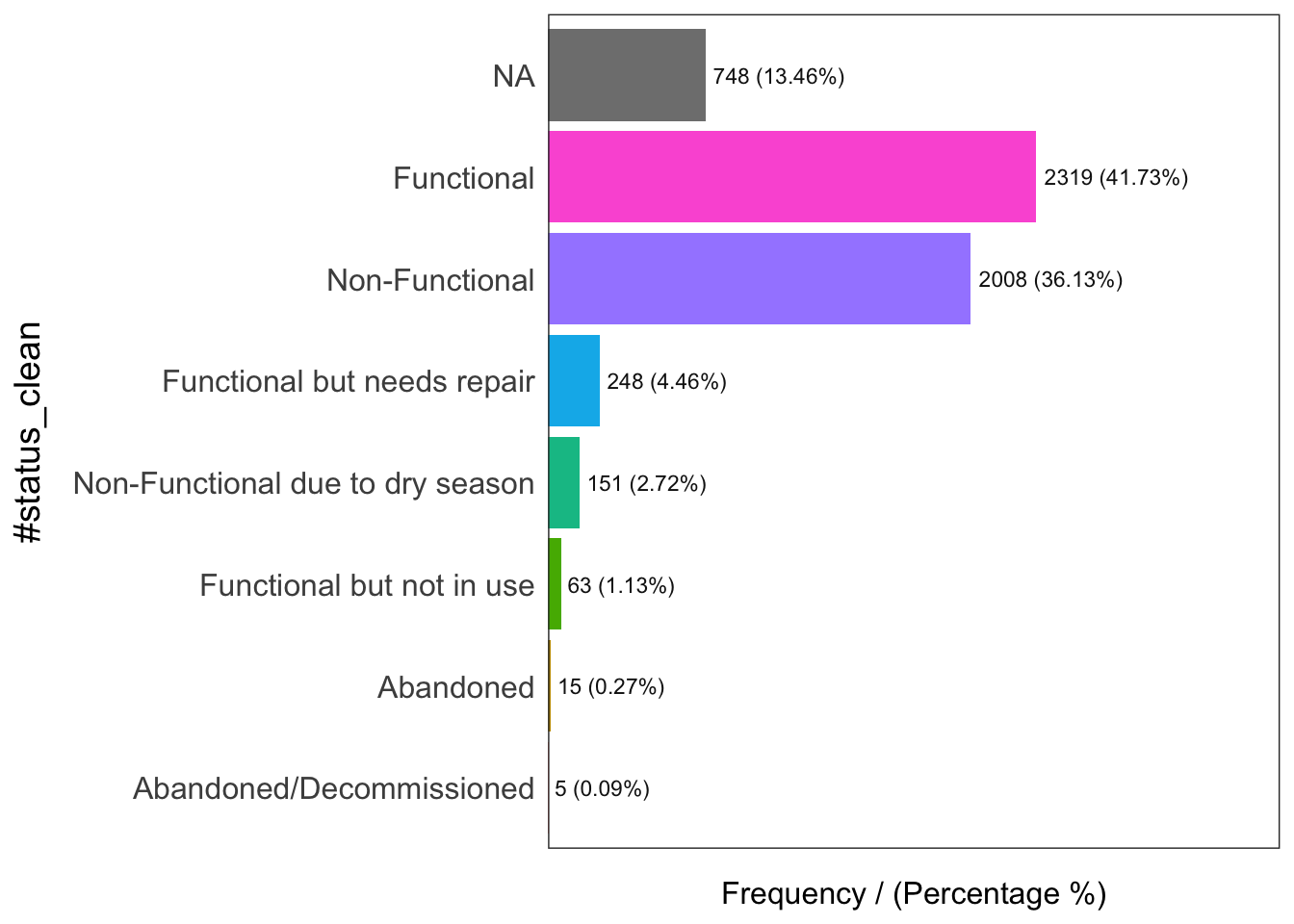
#status_clean frequency percentage cumulative_perc
1 Functional 2319 41.73 41.73
2 Non-Functional 2008 36.13 77.86
3 <NA> 748 13.46 91.32
4 Functional but needs repair 248 4.46 95.78
5 Non-Functional due to dry season 151 2.72 98.50
6 Functional but not in use 63 1.13 99.63
7 Abandoned 15 0.27 99.90
8 Abandoned/Decommissioned 5 0.09 100.00There are eight classes in the #status_clean fields.
To change NA with “unknown”
wp_sf <- wp_sf %>%
rename(status_clean = '#status_clean') %>%
select(status_clean) %>%
mutate(status_clean = replace_na(
status_clean, "unknown"))3.3.3 Extract Water Points
Functional Points
wp_f <- wp_sf %>%
filter(status_clean %in%
c("Functional",
"Functional but needs repair",
"Functional but not in use"))Non-Functional Points
wp_nf <- wp_sf %>%
filter(status_clean %in%
c("Non-Functional",
"Non-Functional due to dry season",
"Abandoned",
"Abandoned/Decommissioned"))Unknown Status Points
wp_u <- wp_sf %>%
filter(status_clean == "unknown")freq(data = wp_f,
input = 'status_clean')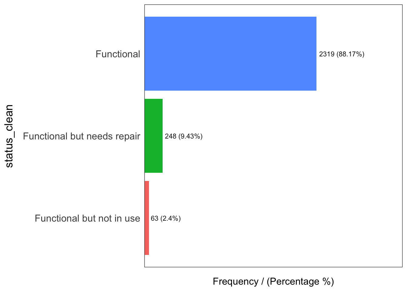
status_clean frequency percentage cumulative_perc
1 Functional 2319 88.17 88.17
2 Functional but needs repair 248 9.43 97.60
3 Functional but not in use 63 2.40 100.00freq(data = wp_nf,
input = 'status_clean')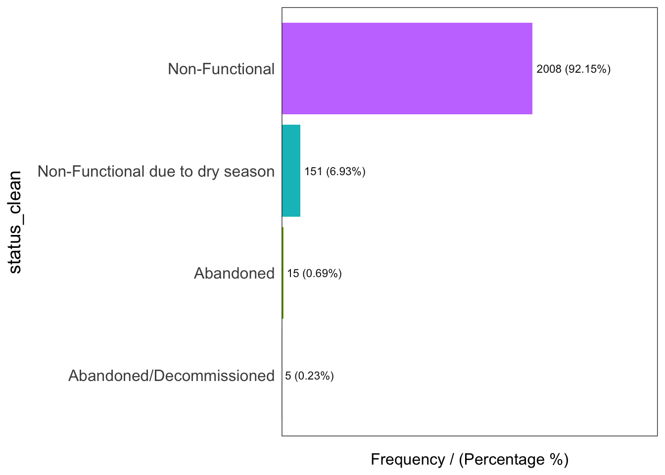
status_clean frequency percentage cumulative_perc
1 Non-Functional 2008 92.15 92.15
2 Non-Functional due to dry season 151 6.93 99.08
3 Abandoned 15 0.69 99.77
4 Abandoned/Decommissioned 5 0.23 100.00freq(data = wp_u,
input = 'status_clean')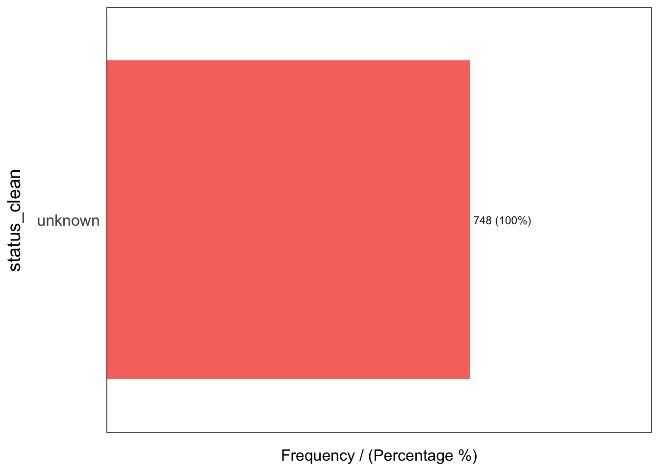
status_clean frequency percentage cumulative_perc
1 unknown 748 100 1003.3.4 Point-in-Polygon Count
Extract number of total, functional, nonfunctional and unknown water points in each local government area (LGA)
wp <- osun %>%
mutate(`total_wp` = lengths(st_intersects(osun, wp_sf))) %>%
mutate(`wp_f` = lengths(st_intersects(osun, wp_f))) %>%
mutate(`wp_nf` = lengths(st_intersects(osun, wp_nf))) %>%
mutate(`wp_u` = lengths(st_intersects(osun, wp_u)))To save as rds format
#write_rds(wp, "Data/rds/wp.rds")ggplot(data = wp,
aes(x = total_wp)) +
geom_histogram(bins=20,
color="black",
fill="light blue") +
geom_vline(aes(xintercept=mean(
total_wp, na.rm=T)),
color="red",
linetype="dashed",
size=0.8) +
ggtitle("Distribution of total water points by LGA") +
xlab("No. of water points") +
ylab("No. of LGAs") 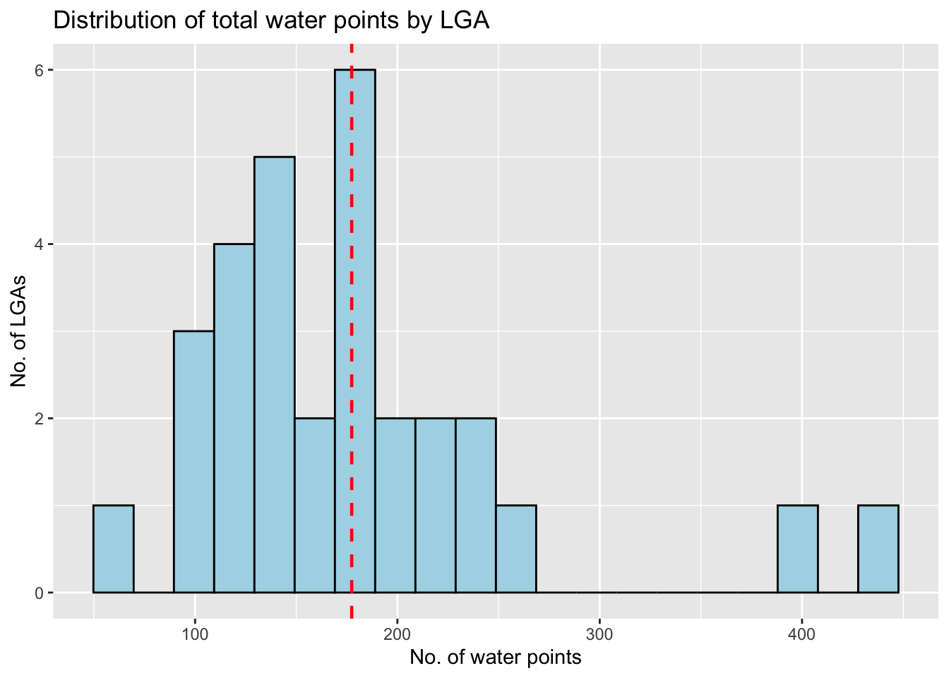
3.4 Combined Data Wrangling
3.4.1 Convert sf dataframes to sp Spatial* class
wp_f_spat = as_Spatial(wp_f)
wp_nf_spat = as_Spatial(wp_nf)
osun_spat = as_Spatial(osun)Peek
wp_f_spatclass : SpatialPointsDataFrame
features : 2630
extent : 177285.9, 290751, 343128.1, 450859.7 (xmin, xmax, ymin, ymax)
crs : +proj=tmerc +lat_0=4 +lon_0=8.5 +k=0.99975 +x_0=670553.98 +y_0=0 +a=6378249.145 +rf=293.465 +towgs84=-92,-93,122,0,0,0,0 +units=m +no_defs
variables : 1
names : status_clean
min values : Functional
max values : Functional but not in use wp_nf_spatclass : SpatialPointsDataFrame
features : 2179
extent : 180539, 290616, 340054.1, 450780.1 (xmin, xmax, ymin, ymax)
crs : +proj=tmerc +lat_0=4 +lon_0=8.5 +k=0.99975 +x_0=670553.98 +y_0=0 +a=6378249.145 +rf=293.465 +towgs84=-92,-93,122,0,0,0,0 +units=m +no_defs
variables : 1
names : status_clean
min values : Abandoned
max values : Non-Functional due to dry season osun_spatclass : SpatialPolygonsDataFrame
features : 30
extent : 176503.2, 291043.8, 331434.7, 454520.1 (xmin, xmax, ymin, ymax)
crs : +proj=tmerc +lat_0=4 +lon_0=8.5 +k=0.99975 +x_0=670553.98 +y_0=0 +a=6378249.145 +rf=293.465 +towgs84=-92,-93,122,0,0,0,0 +units=m +no_defs
variables : 4
names : ADM2_EN, ADM2_PCODE, ADM1_EN, ADM1_PCODE
min values : Aiyedade, NG030001, Osun, NG030
max values : Osogbo, NG030030, Osun, NG030 3.4.2 Convert sp Spatial* class to generic sp format
wp_f_sp <- as(wp_f_spat, "SpatialPoints")
wp_nf_sp <- as(wp_nf_spat, "SpatialPoints")
osun_sp <-as(osun_spat, "SpatialPolygons")Peek
wp_f_spclass : SpatialPoints
features : 2630
extent : 177285.9, 290751, 343128.1, 450859.7 (xmin, xmax, ymin, ymax)
crs : +proj=tmerc +lat_0=4 +lon_0=8.5 +k=0.99975 +x_0=670553.98 +y_0=0 +a=6378249.145 +rf=293.465 +towgs84=-92,-93,122,0,0,0,0 +units=m +no_defs wp_nf_spclass : SpatialPoints
features : 2179
extent : 180539, 290616, 340054.1, 450780.1 (xmin, xmax, ymin, ymax)
crs : +proj=tmerc +lat_0=4 +lon_0=8.5 +k=0.99975 +x_0=670553.98 +y_0=0 +a=6378249.145 +rf=293.465 +towgs84=-92,-93,122,0,0,0,0 +units=m +no_defs osun_spclass : SpatialPolygons
features : 30
extent : 176503.2, 291043.8, 331434.7, 454520.1 (xmin, xmax, ymin, ymax)
crs : +proj=tmerc +lat_0=4 +lon_0=8.5 +k=0.99975 +x_0=670553.98 +y_0=0 +a=6378249.145 +rf=293.465 +towgs84=-92,-93,122,0,0,0,0 +units=m +no_defs 3.4.3 Convert generic sp to spatstat ppp format
# from sp object, convert into ppp format
wp_f_ppp <- as(wp_f_sp, "ppp")
wp_nf_ppp <- as(wp_nf_sp, "ppp")View
par(mfrow=c(1,2))
plot(wp_f_ppp, main="Functional Water Points")
plot(wp_nf_ppp, main="Non-functional Water Points")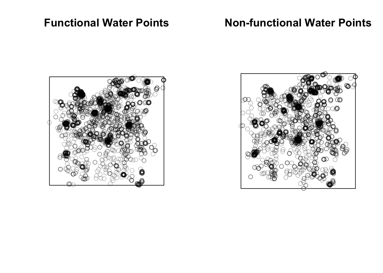
3.4.3.1 Check for Duplication
any(duplicated(wp_f_ppp)); any(duplicated(wp_nf_ppp)) [1] FALSE[1] FALSENo duplicates 🤝 no jittering
3.4.4 Create Owin object
osun_owin <- as(osun_sp, "owin")
plot(osun_owin, main="Owin object of Osun State")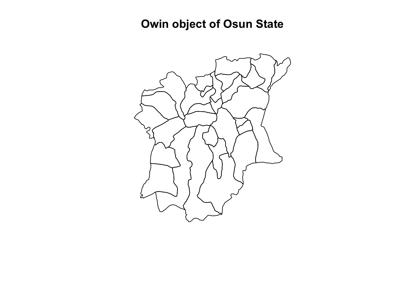
3.4.4 Combine point event object with Owin object
wp_f_ppp = wp_f_ppp[osun_owin]
wp_nf_ppp = wp_nf_ppp[osun_owin]View
Code
par(mfrow=c(1,2))
plot(wp_f_ppp, main="Functional Water Points")
plot(wp_nf_ppp, main="Non-functional Water Points")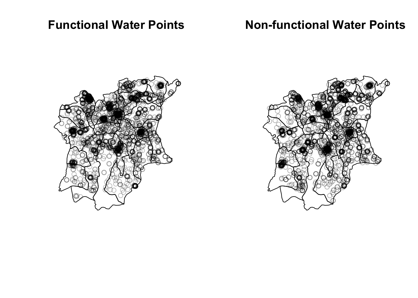
4.0 Exploratory Spatial Data Analysis (ESDA)
4.1 Initial Visualization
Code
wp_f_1 <- tm_shape(wp) +
tm_fill("wp_f",
n = 10,
style = "equal",
palette = "Blues") +
tm_borders(lwd = 0.1,
alpha = 1) +
tm_layout(title = "Functional Water Points by LGA",
legend.outside = TRUE)
wp_f_2 <- tm_shape(wp) +
tm_fill("wp_nf",
n = 10,
style = "equal",
palette = "Blues") +
tm_borders(lwd = 0.1,
alpha = 1) +
tm_layout(title = "Non-functional Water Points by LGA",
legend.outside = TRUE)
tmap_arrange(wp_f_1, wp_f_2, nrow = 1)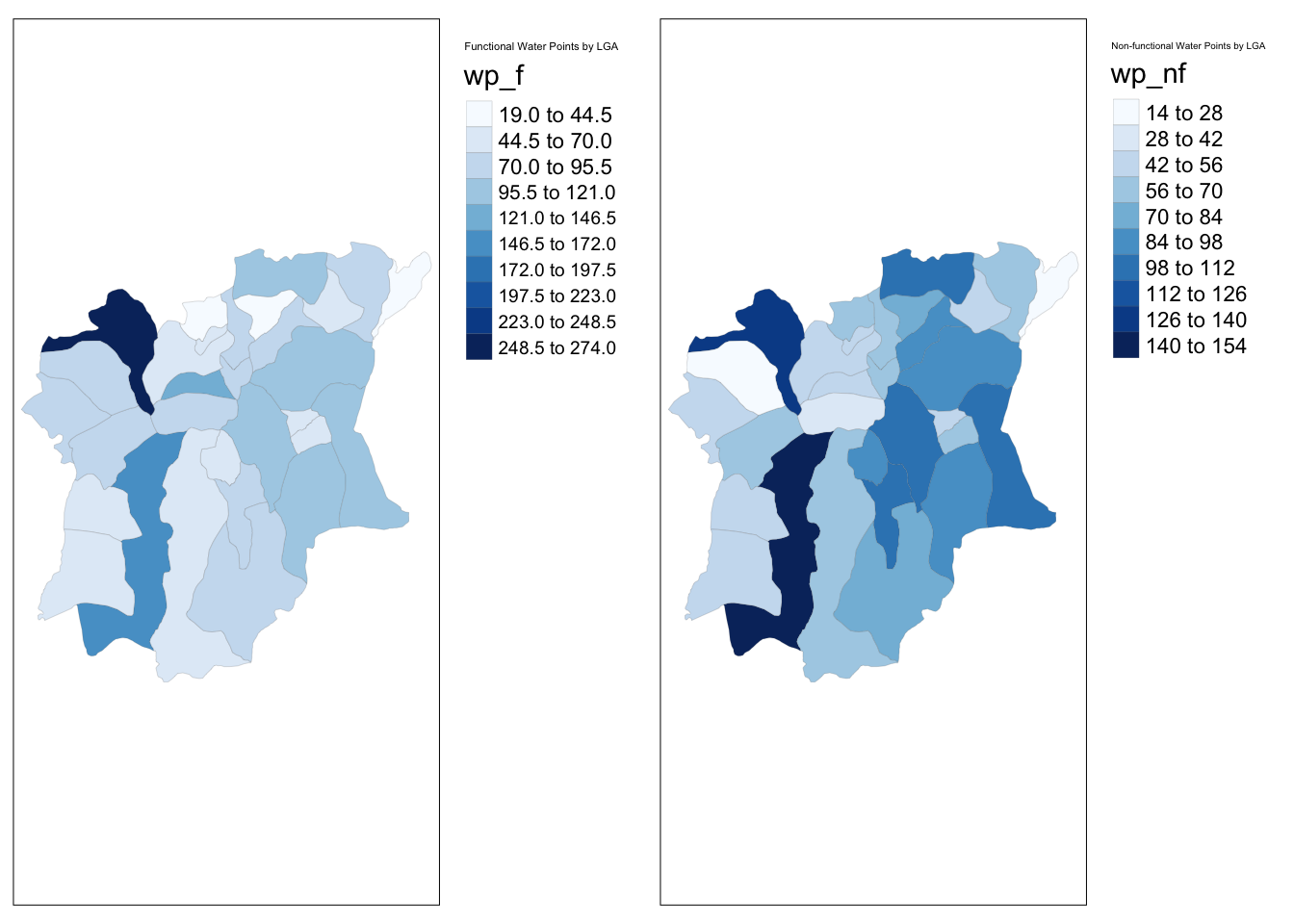
Code
tmap_mode("view") +
tm_basemap("OpenStreetMap") +
tm_shape(wp_f) +
tm_dots(col = "status_clean",
pal = "blue",
border.col = "black",
title = "Functional") +
tm_shape(wp_nf) +
tm_dots(col = "status_clean",
pal = "purple",
border.col = "black",
title = "Non-Functional") +
tm_view(set.bounds = c(4,7,5,8),
set.zoom.limits = c(8,15)) 4.1 Kernel Density Estimation (KDE)
Sigma = bw.ppl() is used as there are multiple clusters and would be more prominent than bw.diggle()
kde_wp_f <- density(wp_f_ppp,
sigma=bw.ppl,
edge=TRUE,
kernel = "gaussian")
kde_wp_nf <- density(wp_nf_ppp,
sigma=bw.ppl,
edge=TRUE,
kernel = "gaussian")
par(mfrow=c(1,2))
plot(kde_wp_f,
main = "Functional Water Points (in m)",
ribside=c("bottom"))
plot(kde_wp_nf,
main = "Non-Functional Water Points (in m)",
ribside=c("bottom"))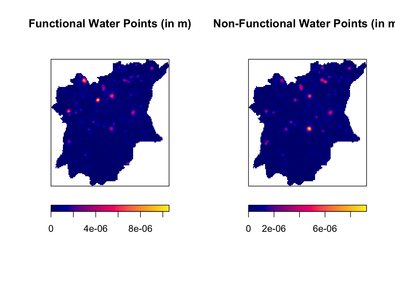
kde_wp_f_ad <- adaptive.density(wp_f_ppp,
method = "kernel")
kde_wp_nf_ad <- adaptive.density(wp_nf_ppp,
method = "kernel")
par(mfrow=c(1,2))
plot(kde_wp_f_ad,
main = "Functional Water Points (in m)",
ribside=c("bottom"))
plot(kde_wp_nf_ad,
main = "Non-Functional Water Points (in m)",
ribside=c("bottom"))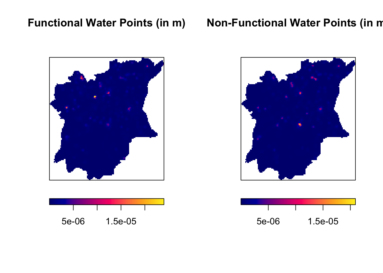
4.2.1 Re-Scale KDE values
From m to km
wp_f_ppp.km <- rescale(wp_f_ppp, 1000, "km")
wp_nf_ppp.km <- rescale(wp_nf_ppp, 1000, "km")kde_wp_f_scale <- density(wp_f_ppp.km,
sigma = bw.ppl,
edge = TRUE)
kde_wp_nf_scale <- density(wp_f_ppp.km,
sigma = bw.ppl,
edge = TRUE)
par(mfrow=c(1,2))
plot(kde_wp_f_scale,
main = "Functional Water Points (in km)",
ribside=c("bottom"))
plot(kde_wp_nf_scale,
main = "Non-Functional Water Points (in km)",
ribside=c("bottom"))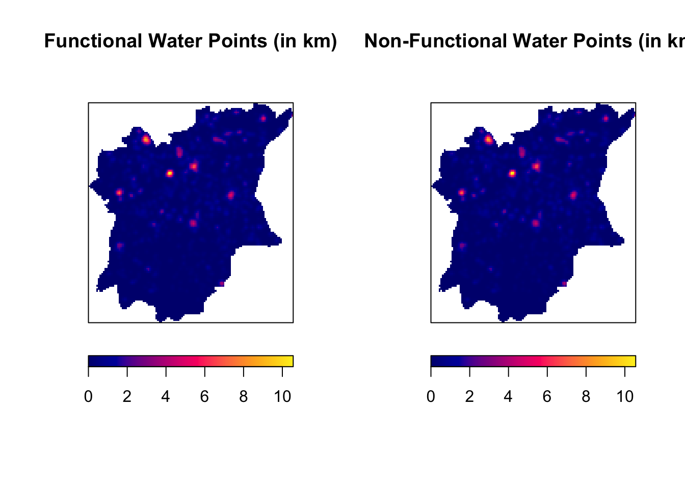
kde_wp_f_scale_ad <- adaptive.density(wp_f_ppp.km,
method = "kernel")
kde_wp_nf_scale_ad <- adaptive.density(wp_nf_ppp.km,
method = "kernel")
par(mfrow=c(1,2))
plot(kde_wp_f_scale_ad,
main = "Functional Water Points (in km)",
ribside=c("bottom"))
plot(kde_wp_nf_scale_ad,
main = "Non-Functional Water Points (in km)",
ribside=c("bottom"))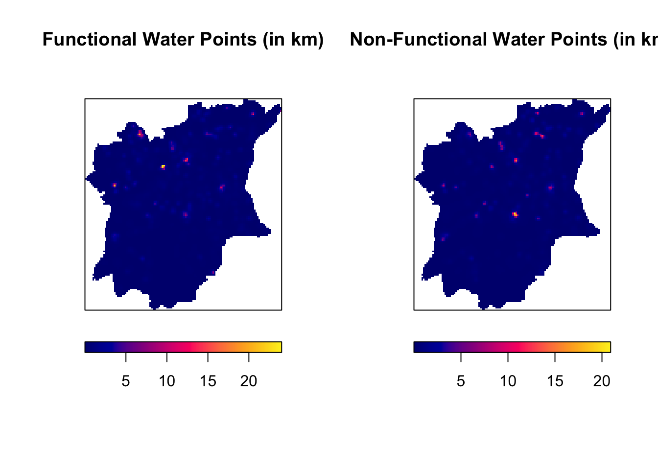
4.2.2 Convert KDE to Grid Object
grid_wp_f <- as.SpatialGridDataFrame.im(kde_wp_f_scale)
grid_wp_nf <- as.SpatialGridDataFrame.im(kde_wp_nf_scale)
spplot(grid_wp_f)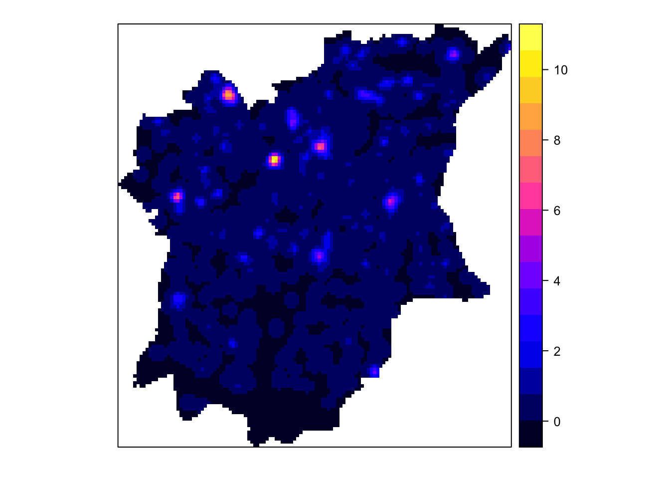
spplot(grid_wp_nf)
grid_wp_f_ad <- as.SpatialGridDataFrame.im(kde_wp_f_scale_ad)
grid_wp_nf_ad <- as.SpatialGridDataFrame.im(kde_wp_nf_scale_ad)
spplot(grid_wp_f_ad)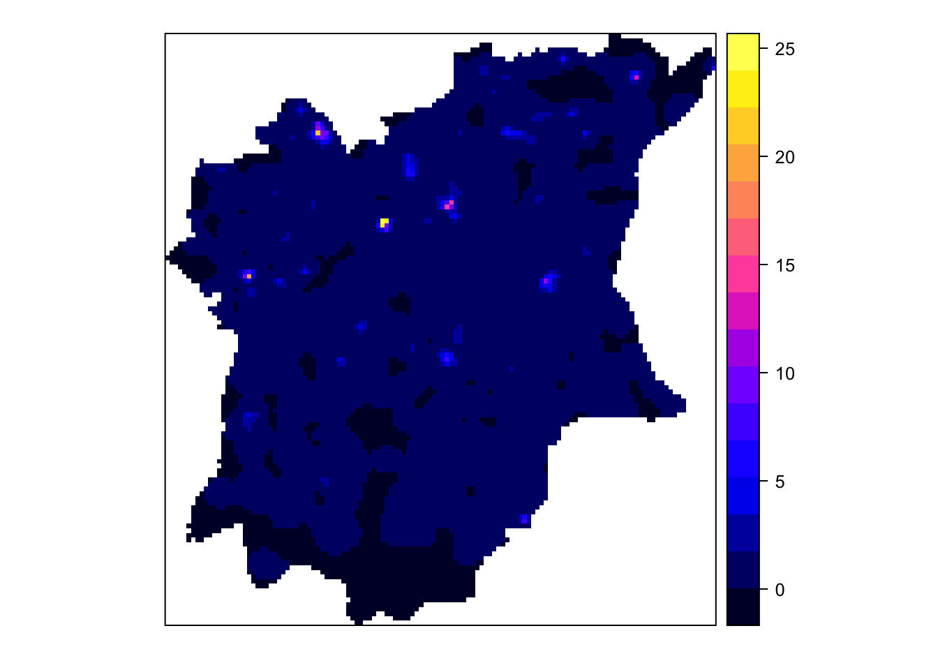
spplot(grid_wp_nf_ad)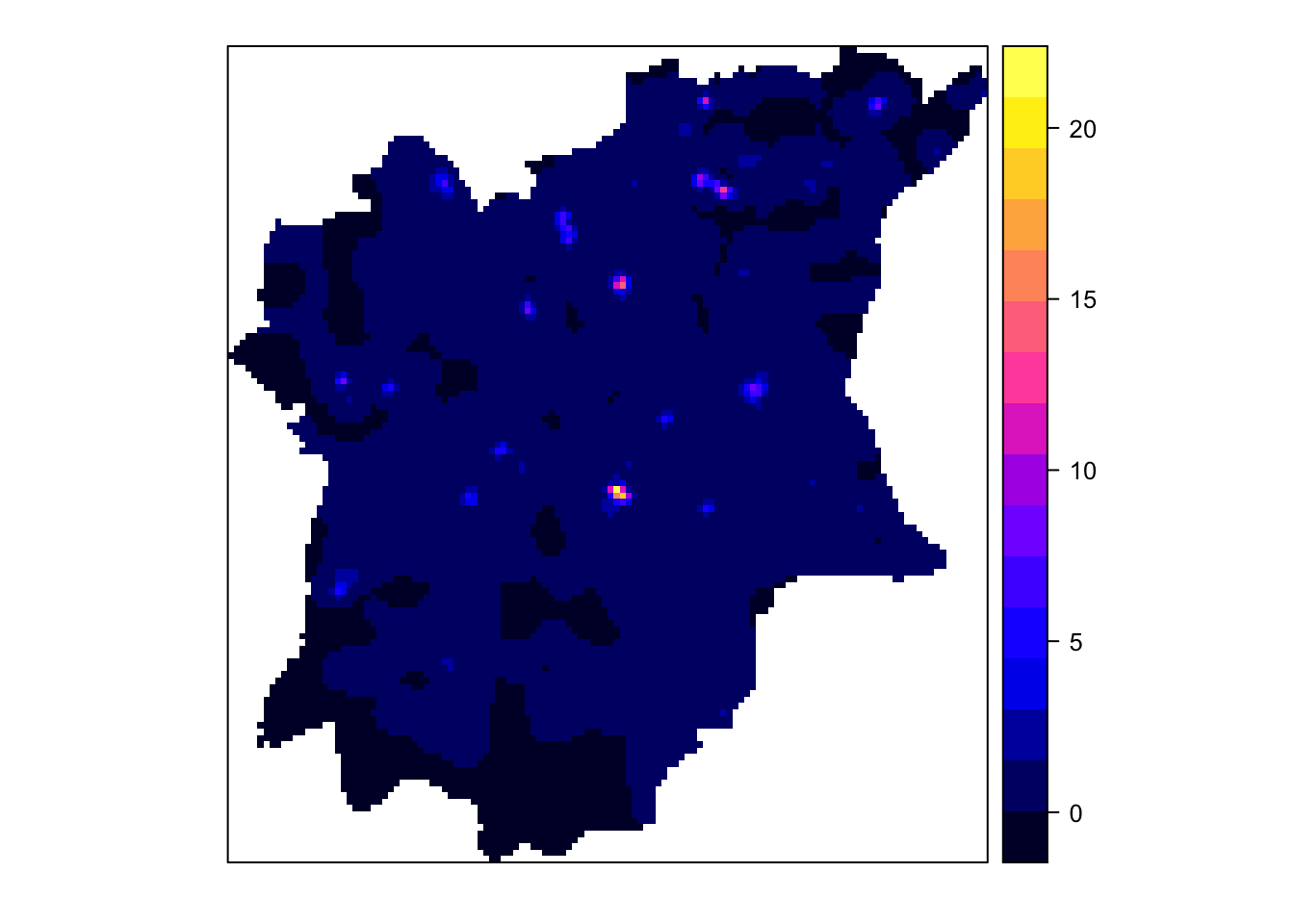
4.2.3 Convert grid object to Raster
kde_wp_f_raster <- raster(grid_wp_f)
kde_wp_f_rasterclass : RasterLayer
dimensions : 128, 128, 16384 (nrow, ncol, ncell)
resolution : 0.8948485, 0.9616045 (x, y)
extent : 176.5032, 291.0438, 331.4347, 454.5201 (xmin, xmax, ymin, ymax)
crs : NA
source : memory
names : v
values : -3.56348e-16, 10.55944 (min, max)kde_wp_nf_raster <- raster(grid_wp_nf)
kde_wp_nf_rasterclass : RasterLayer
dimensions : 128, 128, 16384 (nrow, ncol, ncell)
resolution : 0.8948485, 0.9616045 (x, y)
extent : 176.5032, 291.0438, 331.4347, 454.5201 (xmin, xmax, ymin, ymax)
crs : NA
source : memory
names : v
values : -3.56348e-16, 10.55944 (min, max)4.2.4 Assign Projection System
projection(kde_wp_f_raster) <- CRS("+init=EPSG:26391 +datum:WGS84 +units=km")
kde_wp_f_rasterclass : RasterLayer
dimensions : 128, 128, 16384 (nrow, ncol, ncell)
resolution : 0.8948485, 0.9616045 (x, y)
extent : 176.5032, 291.0438, 331.4347, 454.5201 (xmin, xmax, ymin, ymax)
crs : +init=EPSG:26391 +datum:WGS84 +units=km
source : memory
names : v
values : -3.56348e-16, 10.55944 (min, max)projection(kde_wp_nf_raster) <- CRS("+init=EPSG:26391 +datum:WGS84 +units=km")
kde_wp_nf_rasterclass : RasterLayer
dimensions : 128, 128, 16384 (nrow, ncol, ncell)
resolution : 0.8948485, 0.9616045 (x, y)
extent : 176.5032, 291.0438, 331.4347, 454.5201 (xmin, xmax, ymin, ymax)
crs : +init=EPSG:26391 +datum:WGS84 +units=km
source : memory
names : v
values : -3.56348e-16, 10.55944 (min, max)4.2 Visualize KDE
Code
#tmap generation function
kde <- function(raster_obj, map_title) {
tmap_mode("view")
#tm_basemap("OpenStreetMap") +
tm_shape(raster_obj) +
tm_raster("v", alpha=0.9, palette = "YlGnBu") +
tm_view(set.bounds = c(4,7,5,8),
set.zoom.limits = c(8, 13))
} kde(kde_wp_f_raster)kde(kde_wp_nf_raster)4.3 Nearest Neighbor Index
Clarke-Evans Test to check if distribution is random, clustered or dispersed with a 95% confidence interval
4.3.1 Test - Functional Water Points
The test hypotheses for Functional Water Point is :
H0 : The distribution is random
H1 : The distribution is not random
clarkevans.test(wp_f_ppp,
correction="none",
clipregion=NULL,
alternative=c("clustered"),
nsim=99)
Clark-Evans test
No edge correction
Monte Carlo test based on 99 simulations of CSR with fixed n
data: wp_f_ppp
R = 0.44265, p-value = 0.01
alternative hypothesis: clustered (R < 1)4.3.2 Test - Non-Functional Water Points
The test hypotheses for Non-Functional Water Point is :
H0 : The distribution is random
H1 : The distribution is not random (clustered)
clarkevans.test(wp_nf_ppp,
correction="none",
clipregion=NULL,
alternative=c("clustered"),
nsim=99)
Clark-Evans test
No edge correction
Monte Carlo test based on 99 simulations of CSR with fixed n
data: wp_nf_ppp
R = 0.43223, p-value = 0.01
alternative hypothesis: clustered (R < 1)4.3.3 Conclusion
As the p-value is less than 0.05 is statistically significant and R<1 for both functional and non-functional water points, we reject the null hypothesis that the distribution is not random and conclude that the water points are likely clustered.
5.0 2nd Order Spatial Point Pattern Analysis
Using G-Function for analysis with 95% confidence
5.1 Test 1 - Functional Water Points
The test hypotheses for Functional Water Point is :
H0 : The distribution is random
H1 : The distribution is not random
G_wp_f = Gest(wp_f_ppp, correction = "border")
plot(G_wp_f)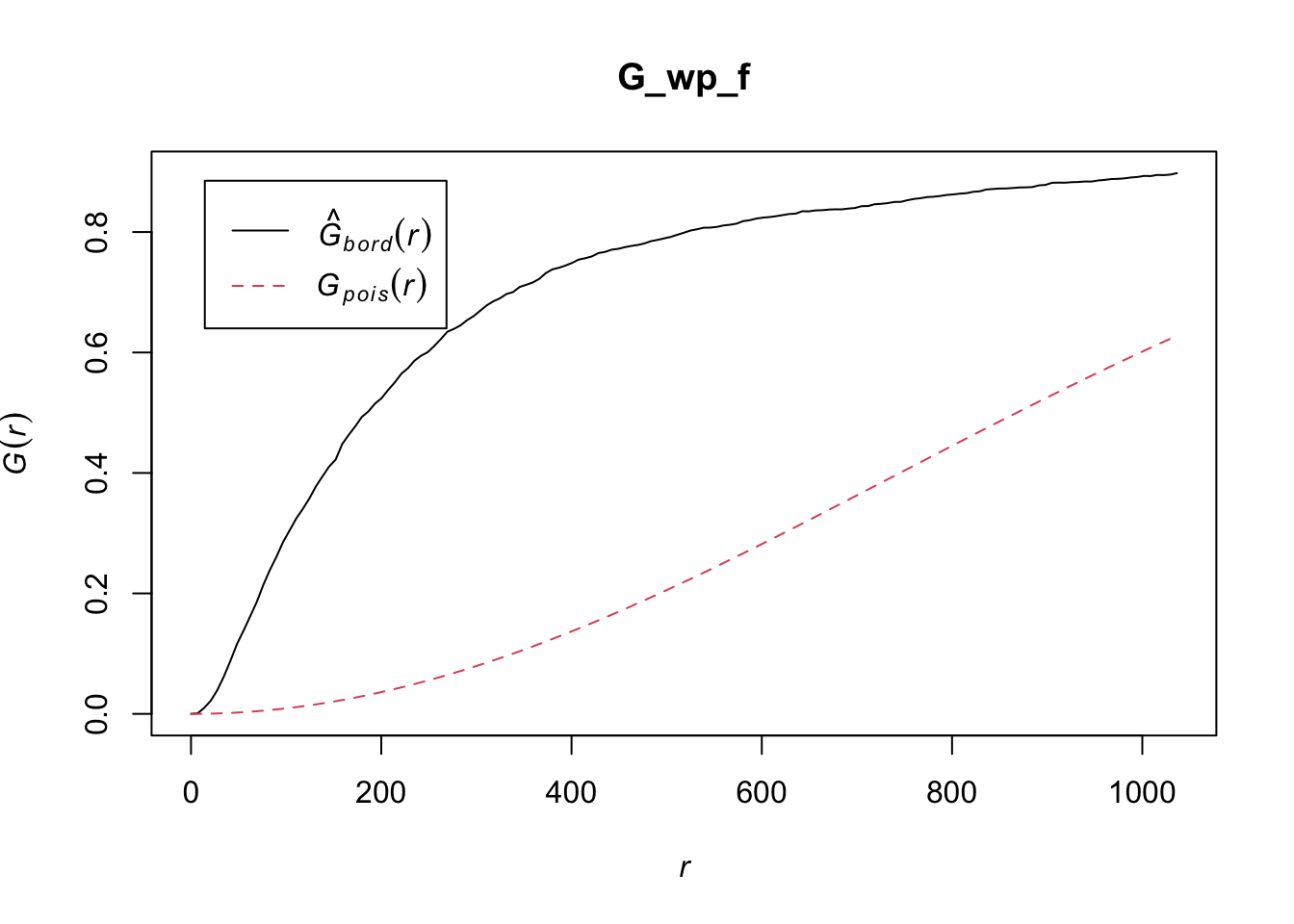
Complete Spatial Randomness Test
G_wp_f.csr <- envelope(wp_f_ppp, Gest, nsim = 500)Generating 500 simulations of CSR ...
1, 2, 3, .5....10....15....20....25....30....35....40....45....50....55...
.60....65....70....75....80....85....90....95....100....105....110....115.
...120....125....130....135....140....145....150....155....160....165....170....
175....180....185....190....195....200....205....210....215....220....225....230..
..235....240....245....250....255....260....265....270....275....280....285....290
....295....300....305....310....315....320....325....330....335....340....345...
.350....355....360....365....370....375....380....385....390....395....400....405.
...410....415....420....425....430....435....440....445....450....455....460....
465....470....475....480....485....490....495.... 500.
Done.plot(G_wp_f.csr, main="G test - Functional")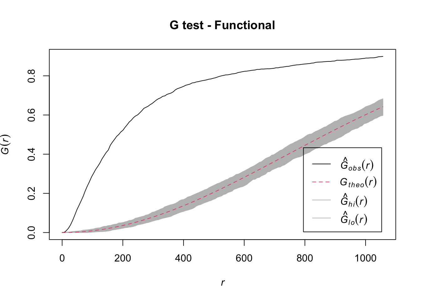
5.1.1 Conclusion
We reject the null hypothesis that functional water points are randomly distributed at 99% confidence interval. As G^obs(r) rises quickly and is greater than Gtheo(r) and the envelope it means the functional water points are clustered.
5.2 Test 2 - Non-functional Water Points
The test hypotheses for Non-Functional Water Point is :
H0 : The distribution is random
H1 : The distribution is not random
G_wp_nf = Gest(wp_nf_ppp, correction = "border")
plot(G_wp_nf)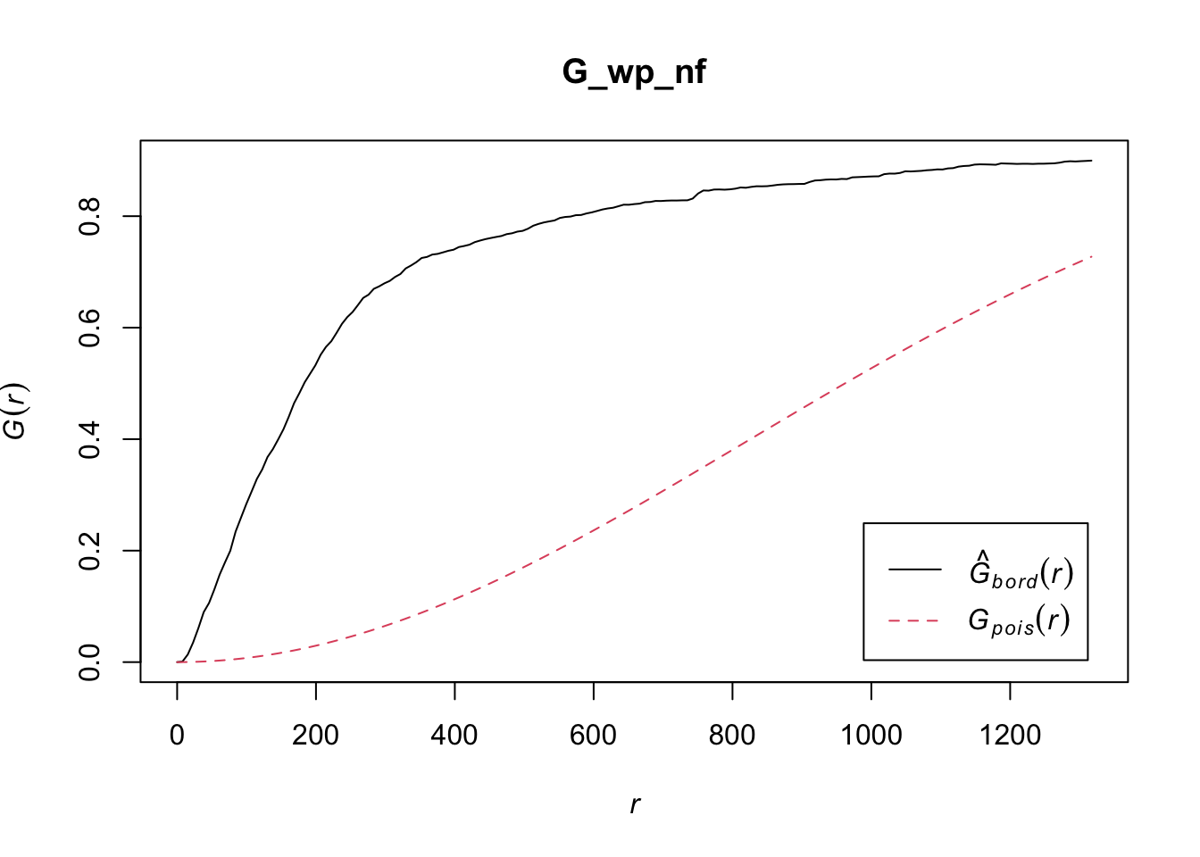
Complete Spatial Randomness Test
G_wp_nf.csr <- envelope(wp_nf_ppp, Gest, nsim = 500)Generating 500 simulations of CSR ...
1, 2, 3, .5....10....15....20....25....30....35....40....45....50....55...
.60....65....70....75....80....85....90....95....100....105....110....115.
...120....125....130....135....140....145....150....155....160....165....170....
175....180....185....190....195....200....205....210....215....220....225....230..
..235....240....245....250....255....260....265....270....275....280....285....290
....295....300....305....310....315....320....325....330....335....340....345...
.350....355....360....365....370....375....380....385....390....395....400....405.
...410....415....420....425....430....435....440....445....450....455....460....
465....470....475....480....485....490....495.... 500.
Done.plot(G_wp_nf.csr, main = "G test - Non-functional")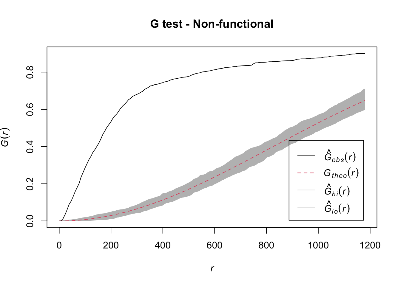
5.2.1 Conclusion
We reject the null hypothesis that non-functional water points are randomly distributed at 99% confidence interval. As G^obs(r) rises quickly and is greater than Gtheo(r) and the envelope it means the functional water points are clustered.
5.3 Extra Tests
We see the same observation as mentioned above after zooming into a few neighborhoods such as Ife Central for functional water ponits and Ede North for non-functional water points.
5.3.1 Data Processing
#Functional water points
IfeCentral <- osun[osun$ADM2_EN == "Ife Central",] %>%
as('Spatial') %>%
as('SpatialPolygons') %>%
as('owin')
#non functional points
EdeNorth <- osun[osun$ADM2_EN == "Ede North",] %>%
as('Spatial') %>%
as('SpatialPolygons') %>%
as('owin')
IfeCentral_ppp <- wp_f_ppp[IfeCentral]
EdeNorth_ppp <- wp_nf_ppp[EdeNorth]View
Code
par(mfrow=c(1,2))
plot(IfeCentral_ppp,
main = "Ife Central - Functional Water Points",
ribside=c("bottom"))
plot(EdeNorth_ppp,
main = "Ede North - Non-Functional Water Points",
ribside=c("bottom"))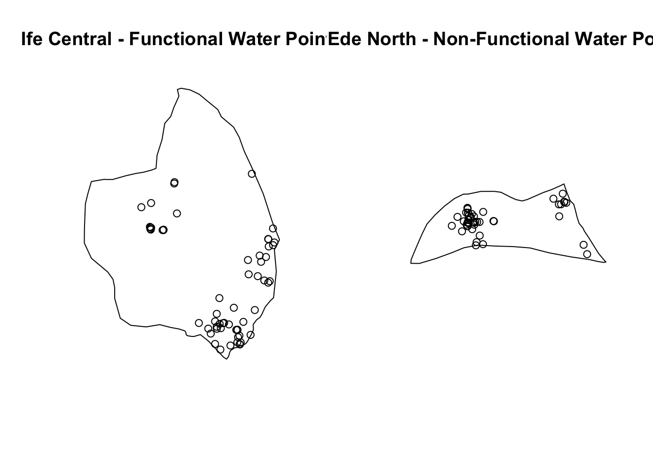
5.3.2 Ife Central - Functional Water Points
Ifecentral_G.csr = Gest(IfeCentral_ppp, correction = "border")
plot(Ifecentral_G.csr)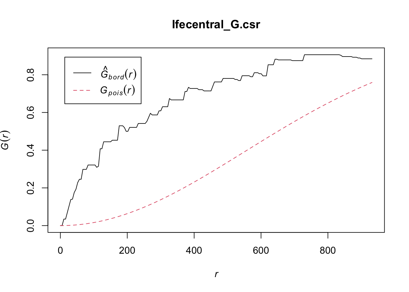
Complete Spatial Randomness Test
Ifecentral_G.csr <- envelope(IfeCentral_ppp, Gest, nsim=100)Generating 100 simulations of CSR ...
1, 2, 3, 4, 5, 6, 7, 8, 9, 10, 11, 12, 13, 14, 15, 16, 17, 18, 19, 20, 21, 22, 23, 24, 25, 26, 27, 28, 29, 30, 31, 32, 33, 34, 35, 36, 37, 38, 39, 40,
41, 42, 43, 44, 45, 46, 47, 48, 49, 50, 51, 52, 53, 54, 55, 56, 57, 58, 59, 60, 61, 62, 63, 64, 65, 66, 67, 68, 69, 70, 71, 72, 73, 74, 75, 76, 77, 78, 79, 80,
81, 82, 83, 84, 85, 86, 87, 88, 89, 90, 91, 92, 93, 94, 95, 96, 97, 98, 99, 100.
Done.plot(Ifecentral_G.csr, main="Ife Central G-Function Test")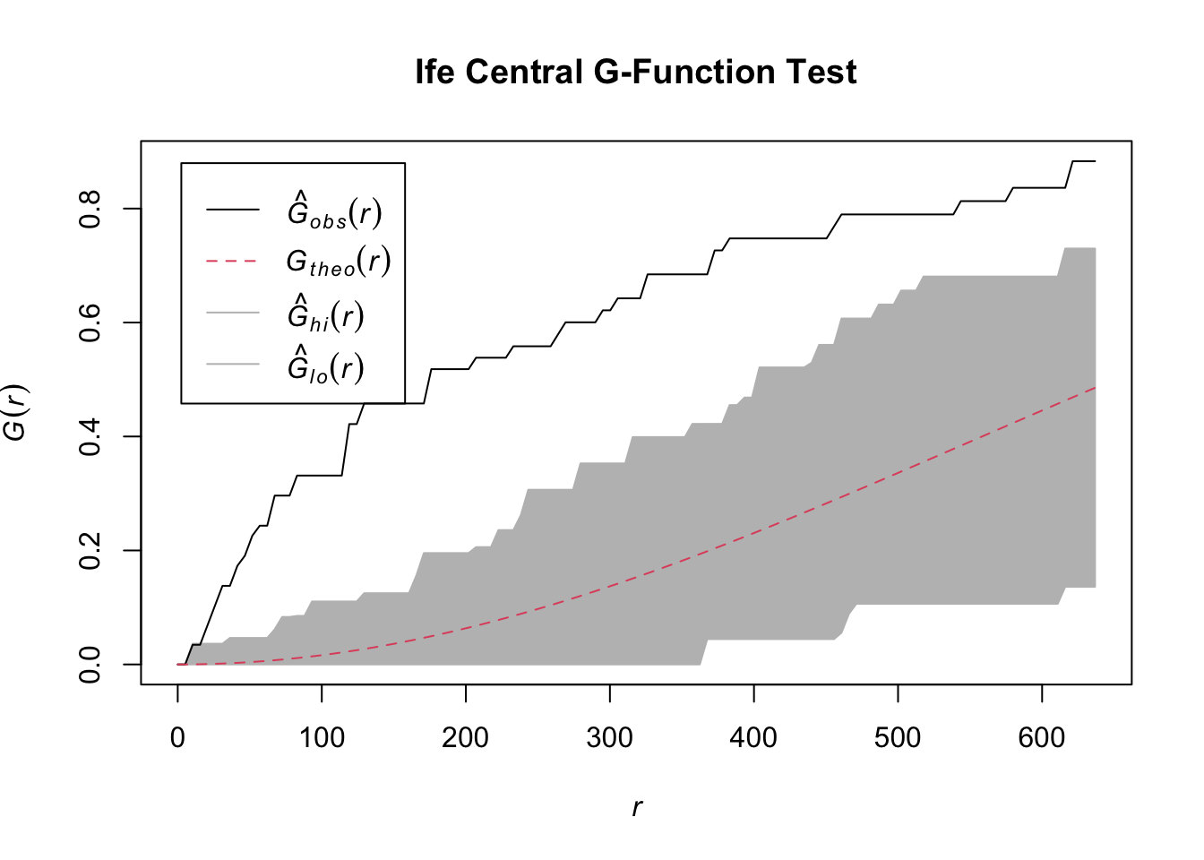
5.3.3 Ede North - Non-Functional Water Points
EdeNorth_G.csr = Gest(EdeNorth_ppp, correction = "border")
plot(EdeNorth_G.csr)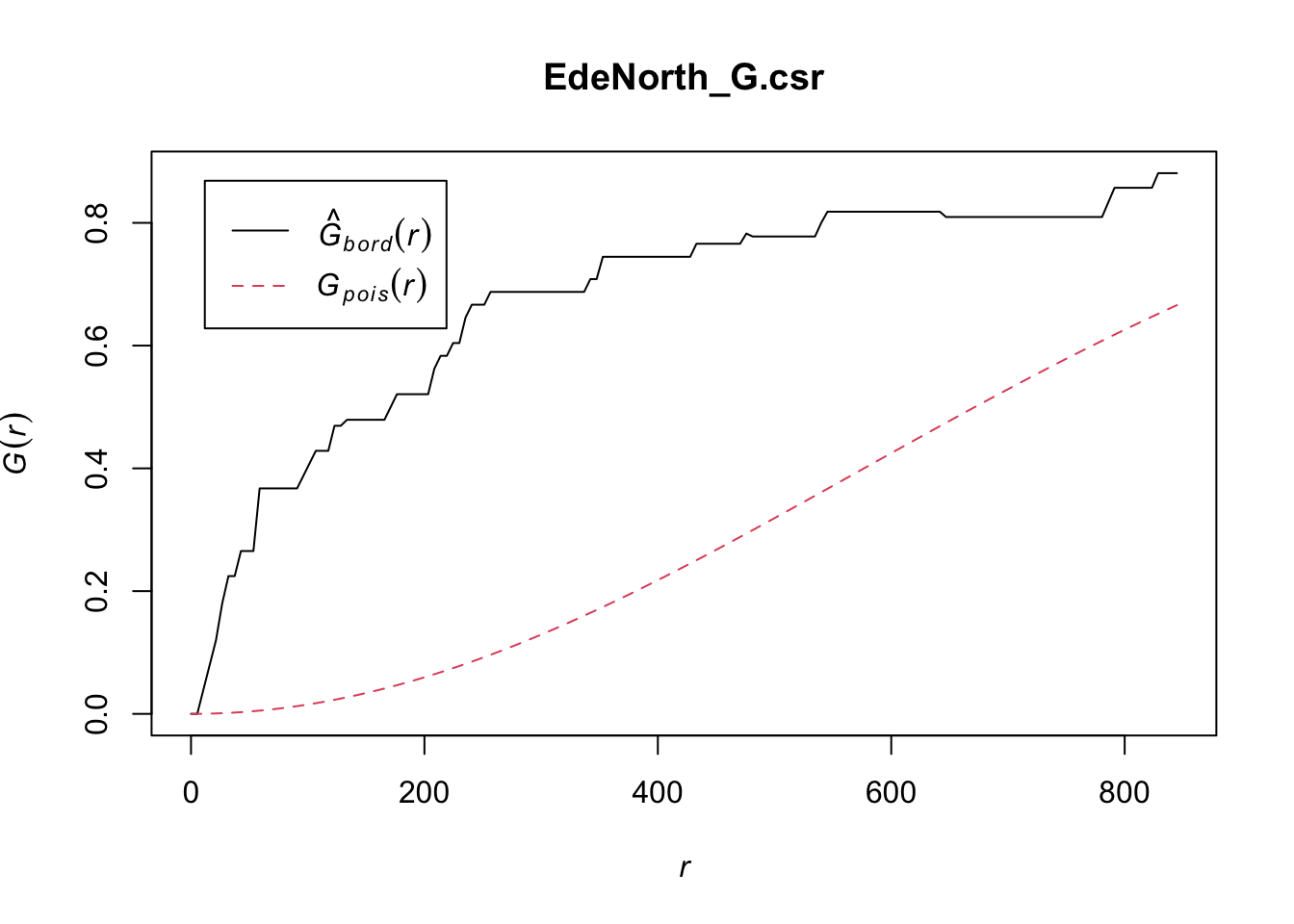
Complete Spatial Randomness Test
EdeNorth_G.csr <- envelope(EdeNorth_ppp, Gest, nsim=100)Generating 100 simulations of CSR ...
1, 2, 3, 4, 5, 6, 7, 8, 9, 10, 11, 12, 13, 14, 15, 16, 17, 18, 19, 20, 21, 22, 23, 24, 25, 26, 27, 28, 29, 30, 31, 32, 33, 34, 35, 36, 37, 38, 39, 40,
41, 42, 43, 44, 45, 46, 47, 48, 49, 50, 51, 52, 53, 54, 55, 56, 57, 58, 59, 60, 61, 62, 63, 64, 65, 66, 67, 68, 69, 70, 71, 72, 73, 74, 75, 76, 77, 78, 79, 80,
81, 82, 83, 84, 85, 86, 87, 88, 89, 90, 91, 92, 93, 94, 95, 96, 97, 98, 99, 100.
Done.plot(EdeNorth_G.csr, main="Ede North G-Function Test")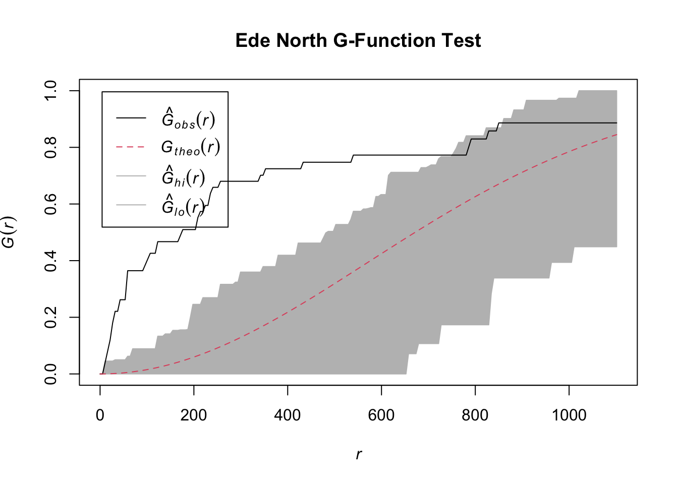
5.3.4 Conclusion
We observe the same that G^obs(r) rises quickly and is greater than Gtheo(r) and the envelope it means the functional and non-functional water points are clustered, thereby rejecting the null hypothesis that the water points are randomly distributed at 99% confidence interval.
6.0 Spatial Correlation Analysis
6.1 Density Analysis
Segregate data for plotting. Then convert to spatstat ppp format
wp_spat <- as_Spatial(wp_sf)
wp_spat@data$status_clean <-as.factor(wp_spat@data$status_clean)
wp_spat_ppp <- as(wp_spat, "ppp")
plot(wp_spat_ppp, which.marks = "status_clean")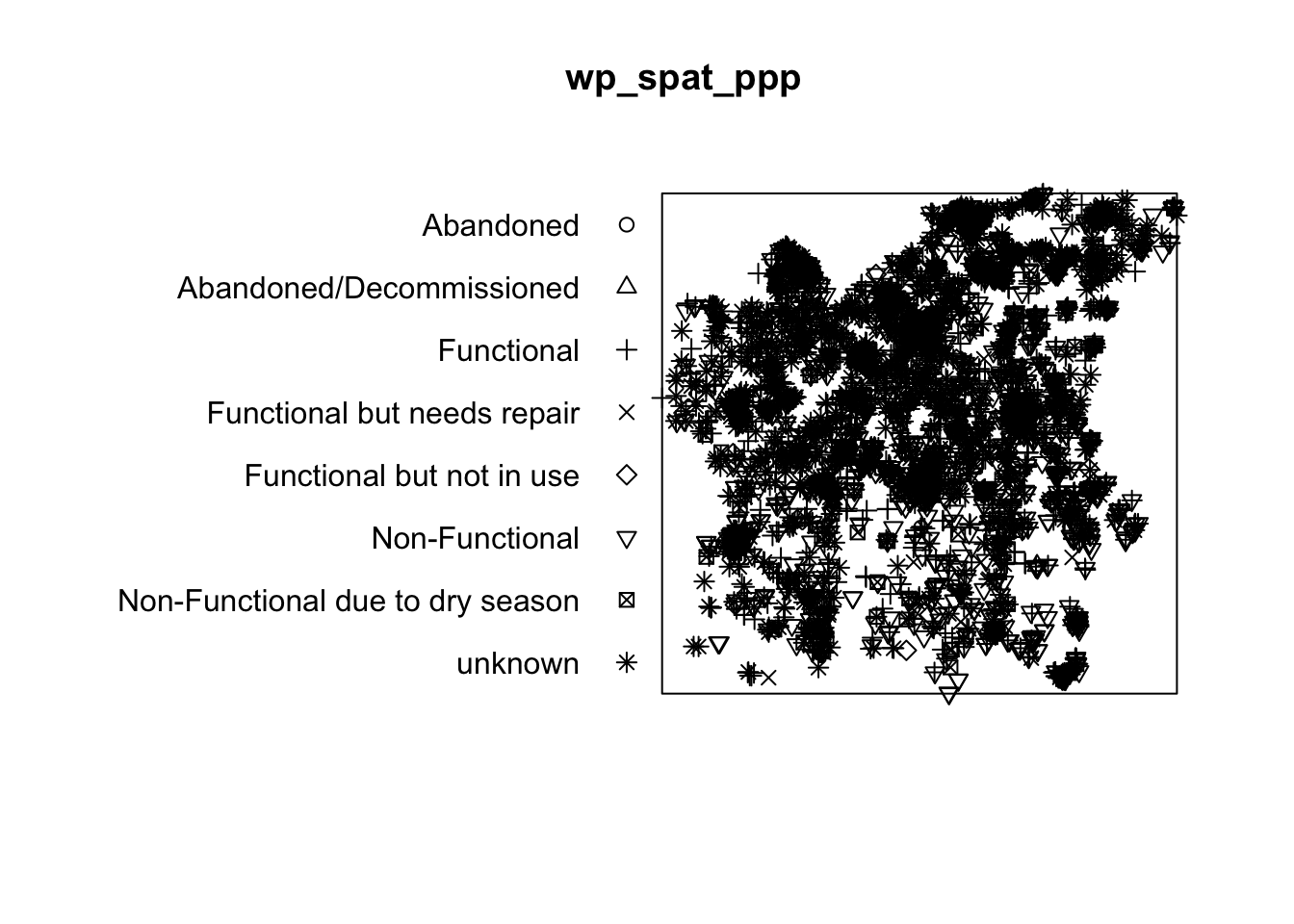
6.3 Test Correlation
Use LCross function to test for spatial independence
The test hypotheses for the spatial distribution of functional and non-functional water point are:
H0 : The distribution is spatially independent
H1 : The distribution is not spatially independent
Simulation
wp_spat_ppp_Lcross.csr <- envelope(wp_spat_ppp,
Lcross,
i="Functional",
j="Non-Functional",
correction="border",
nsim=100)Generating 100 simulations of CSR ...
1, 2, 3, 4, 5, 6, 7, 8, 9, 10, 11, 12, 13, 14, 15, 16, 17, 18, 19, 20, 21, 22, 23, 24, 25, 26, 27, 28, 29, 30, 31, 32, 33, 34, 35, 36, 37, 38, 39, 40,
41, 42, 43, 44, 45, 46, 47, 48, 49, 50, 51, 52, 53, 54, 55, 56, 57, 58, 59, 60, 61, 62, 63, 64, 65, 66, 67, 68, 69, 70, 71, 72, 73, 74, 75, 76, 77, 78, 79, 80,
81, 82, 83, 84, 85, 86, 87, 88, 89, 90, 91, 92, 93, 94, 95, 96, 97, 98, 99, 100.
Done.Plot
plot(wp_spat_ppp_Lcross.csr, xlab="in km")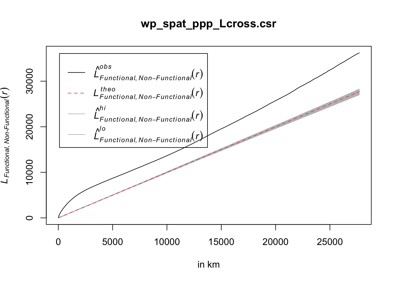
Conclusion
We reject the null hypothesis that water points are statistically independent at 99% confidence interval. As L^obs(r) is greater than Ltheo(r) and the envelope it means the water points are statistically not independent.
6.4 Local Colocation Analysis
Remove status ‘unknown’ water points
wp_sf_clean <- wp_sf %>% filter(!status_clean=='unknown')#6 nearbest neighbors
nb = include_self(st_knn(st_geometry(wp_sf_clean), 6))
#weight matrix
wt = st_kernel_weights(nb, wp_sf_clean, "gaussian", adaptive = TRUE)
f = wp_sf_clean %>%
filter(status_clean == "Functional")
A = f$status_clean
nf = wp_sf_clean %>%
filter(status_clean == "Non-Functional")
B = nf$status_clean
LCLQ = local_colocation(A, B, nb, wt, 42)
LCLQ_wp = cbind(wp_sf_clean, LCLQ)LCLQ_wp <- LCLQ_wp %>%
mutate(
`p_sim_Non.Functional` = replace(`p_sim_Non.Functional`, `p_sim_Non.Functional` > 0.05, NA),
`Non.Functional` = ifelse(`p_sim_Non.Functional` > 0.05, NA, `Non.Functional`))
LCLQ_wp <- LCLQ_wp %>% mutate(`size` = ifelse(is.na(`Non.Functional`), 1, 5))View
Code
tmap_mode('view')
tm_view(set.bounds = c(4,7,5,8),
set.zoom.limits=c(8, 13),
bbox = st_bbox(filter(LCLQ_wp, !is.na(`Non.Functional`)))) +
tm_shape(osun) +
tm_borders() +
tm_shape(LCLQ_wp) +
tm_dots(col = c("Non.Functional"),
size = "size",
scale=0.15,
border.col = "black",
border.lwd = 0.5,
alpha=0.5,
title="LCLQ"
)Code
tmap_mode('plot')LCLQ is just less than 1 which is much greater than the p-value of 0.05. Hence it means there are few Non-Functional Water Points in the same neighborhood as Functional Water Points.
7.0 Acknowledgements
I’d like to thank Professor Kam for his insights and resource materials provided under IS415 Geospatial Analytics and Applications.