pacman::p_load(sf, sfdep, tmap, maptools, kableExtra, plotly, lubridate, tidyr, readxl, tidyverse)Take Home Exercise 2
1.0 Overview
1.1 Background
Due to the COVID-19 outbreak in late December 2019, Indonesia commenced its COVID-19 vaccination program on 13 January 2021. Despite having the 4th highest number of vaccines administered as of January 4th, 2022, the distribution was not necessarily even.
This notebook explore how the vaccination rates changed over time for the DKI Jarkarta on a sub-district level.
1.2 Task
Choropleth Mapping and Analysis
Local Gi* Analysis
Emerging Hot Spot Analysis (EHSA)
2.0 Setup
2.1 Import Packages
sf - Used for handling geospatial data
sfdep - Used for functions not in spdep
tmap, maptools, kableExtra, plotly - Used for visualizing dataframes and plots
lubridate - Used for handling datetime
tidyr - Used for changing the shape and hierarchy of dataframe
readxl - to read excel data (.xlsx files)
tidyVerse - Used for data transformation and presentation
3.0 Data Wrangling
3.1 Datasets Used
| Type | Name |
|---|---|
| Geopsatial | BATAS_DESA_DESEMBER_2019_DUKCAPIL_DKI_JAKARTA |
| Aspatial | DKI Jakarta Provincial Vaccination Open Data |
3.2 Geospatial Data
3.2.1 Load Data
bd_jakarta <- st_read(dsn="data/geospatial",
                      layer="BATAS_DESA_DESEMBER_2019_DUKCAPIL_DKI_JAKARTA")
Reading layer `BATAS_DESA_DESEMBER_2019_DUKCAPIL_DKI_JAKARTA' from data source
`/Users/shambhavigoenka/Desktop/School/Geo/IS415-GAA/take_home_ex/take_home_ex02/data/geospatial'
using driver `ESRI Shapefile'
Simple feature collection with 269 features and 161 fields
Geometry type: MULTIPOLYGON
Dimension: XY
Bounding box: xmin: 106.3831 ymin: -6.370815 xmax: 106.9728 ymax: -5.184322
Geodetic CRS: WGS 84glimpse(bd_jakarta)Rows: 269
Columns: 162
$ OBJECT_ID <dbl> 25477, 25478, 25397, 25400, 25378, 25379, 25390, 25382, 253…
$ KODE_DESA <chr> "3173031006", "3173031007", "3171031003", "3171031006", "31…
$ DESA <chr> "KEAGUNGAN", "GLODOK", "HARAPAN MULIA", "CEMPAKA BARU", "PU…
$ KODE <dbl> 317303, 317303, 317103, 317103, 310101, 310101, 317102, 310…
$ PROVINSI <chr> "DKI JAKARTA", "DKI JAKARTA", "DKI JAKARTA", "DKI JAKARTA",…
$ KAB_KOTA <chr> "JAKARTA BARAT", "JAKARTA BARAT", "JAKARTA PUSAT", "JAKARTA…
$ KECAMATAN <chr> "TAMAN SARI", "TAMAN SARI", "KEMAYORAN", "KEMAYORAN", "KEPU…
$ DESA_KELUR <chr> "KEAGUNGAN", "GLODOK", "HARAPAN MULIA", "CEMPAKA BARU", "PU…
$ JUMLAH_PEN <dbl> 21609, 9069, 29085, 41913, 6947, 7059, 15793, 5891, 33383, …
$ JUMLAH_KK <dbl> 7255, 3273, 9217, 13766, 2026, 2056, 5599, 1658, 11276, 128…
$ LUAS_WILAY <dbl> 0.36, 0.37, 0.53, 0.97, 0.93, 0.95, 1.76, 1.14, 0.47, 1.31,…
$ KEPADATAN <dbl> 60504, 24527, 54465, 42993, 7497, 7401, 8971, 5156, 71628, …
$ PERPINDAHA <dbl> 102, 25, 131, 170, 17, 26, 58, 13, 113, 178, 13, 87, 56, 12…
$ JUMLAH_MEN <dbl> 68, 52, 104, 151, 14, 32, 36, 10, 60, 92, 5, 83, 21, 70, 93…
$ PERUBAHAN <dbl> 20464, 8724, 27497, 38323, 6853, 6993, 15006, 5807, 31014, …
$ WAJIB_KTP <dbl> 16027, 7375, 20926, 30264, 4775, 4812, 12559, 3989, 24784, …
$ SILAM <dbl> 15735, 1842, 26328, 36813, 6941, 7057, 7401, 5891, 23057, 2…
$ KRISTEN <dbl> 2042, 2041, 1710, 3392, 6, 0, 3696, 0, 4058, 5130, 1, 3061,…
$ KHATOLIK <dbl> 927, 1460, 531, 1082, 0, 0, 1602, 0, 2100, 2575, 0, 1838, 7…
$ HINDU <dbl> 15, 9, 42, 127, 0, 0, 622, 0, 25, 27, 0, 9, 115, 47, 382, 7…
$ BUDHA <dbl> 2888, 3716, 469, 495, 0, 2, 2462, 0, 4134, 4740, 5, 1559, 3…
$ KONGHUCU <dbl> 2, 1, 5, 1, 0, 0, 10, 0, 9, 10, 0, 4, 1, 1, 4, 0, 2, 0, 0, …
$ KEPERCAYAA <dbl> 0, 0, 0, 3, 0, 0, 0, 0, 0, 0, 0, 2, 0, 22, 0, 3, 3, 0, 0, 0…
$ PRIA <dbl> 11049, 4404, 14696, 21063, 3547, 3551, 7833, 2954, 16887, 1…
$ WANITA <dbl> 10560, 4665, 14389, 20850, 3400, 3508, 7960, 2937, 16496, 1…
$ BELUM_KAWI <dbl> 10193, 4240, 14022, 20336, 3366, 3334, 7578, 2836, 15860, 1…
$ KAWIN <dbl> 10652, 4364, 13450, 19487, 3224, 3404, 7321, 2791, 15945, 1…
$ CERAI_HIDU <dbl> 255, 136, 430, 523, 101, 80, 217, 44, 381, 476, 39, 305, 10…
$ CERAI_MATI <dbl> 509, 329, 1183, 1567, 256, 241, 677, 220, 1197, 993, 79, 90…
$ U0 <dbl> 1572, 438, 2232, 3092, 640, 648, 802, 585, 2220, 2399, 376,…
$ U5 <dbl> 1751, 545, 2515, 3657, 645, 684, 995, 588, 2687, 2953, 331,…
$ U10 <dbl> 1703, 524, 2461, 3501, 620, 630, 1016, 513, 2653, 2754, 309…
$ U15 <dbl> 1493, 521, 2318, 3486, 669, 671, 1106, 548, 2549, 2666, 328…
$ U20 <dbl> 1542, 543, 2113, 3098, 619, 609, 1081, 491, 2313, 2515, 290…
$ U25 <dbl> 1665, 628, 2170, 3024, 639, 582, 1002, 523, 2446, 2725, 325…
$ U30 <dbl> 1819, 691, 2363, 3188, 564, 592, 1236, 478, 2735, 3122, 329…
$ U35 <dbl> 1932, 782, 2595, 3662, 590, 572, 1422, 504, 3034, 3385, 317…
$ U40 <dbl> 1828, 675, 2371, 3507, 480, 486, 1200, 397, 2689, 3037, 250…
$ U45 <dbl> 1600, 607, 2250, 3391, 421, 457, 1163, 365, 2470, 2597, 206…
$ U50 <dbl> 1408, 619, 1779, 2696, 346, 369, 1099, 288, 2129, 2282, 134…
$ U55 <dbl> 1146, 602, 1379, 1909, 252, 318, 979, 235, 1843, 1930, 129,…
$ U60 <dbl> 836, 614, 1054, 1397, 197, 211, 880, 162, 1386, 1394, 75, 9…
$ U65 <dbl> 587, 555, 654, 970, 122, 114, 747, 111, 958, 932, 50, 706, …
$ U70 <dbl> 312, 311, 411, 631, 69, 55, 488, 65, 554, 573, 38, 412, 129…
$ U75 <dbl> 415, 414, 420, 704, 74, 61, 577, 38, 717, 642, 37, 528, 125…
$ TIDAK_BELU <dbl> 3426, 1200, 4935, 7328, 1306, 1318, 2121, 973, 5075, 6089, …
$ BELUM_TAMA <dbl> 1964, 481, 2610, 3763, 730, 676, 1278, 732, 3241, 3184, 383…
$ TAMAT_SD <dbl> 2265, 655, 2346, 2950, 1518, 2054, 1169, 1266, 4424, 3620, …
$ SLTP <dbl> 3660, 1414, 3167, 5138, 906, 1357, 2236, 852, 5858, 6159, 5…
$ SLTA <dbl> 8463, 3734, 12172, 16320, 2040, 1380, 5993, 1570, 12448, 14…
$ DIPLOMA_I <dbl> 81, 23, 84, 179, 22, 15, 43, 36, 85, 83, 4, 63, 27, 79, 110…
$ DIPLOMA_II <dbl> 428, 273, 1121, 1718, 101, 59, 573, 97, 604, 740, 25, 734, …
$ DIPLOMA_IV <dbl> 1244, 1241, 2477, 4181, 314, 191, 2199, 357, 1582, 1850, 83…
$ STRATA_II <dbl> 74, 46, 166, 315, 10, 8, 168, 8, 63, 92, 5, 174, 125, 122, …
$ STRATA_III <dbl> 4, 2, 7, 21, 0, 1, 13, 0, 3, 9, 0, 16, 8, 7, 75, 49, 65, 14…
$ BELUM_TIDA <dbl> 3927, 1388, 5335, 8105, 1788, 1627, 2676, 1129, 5985, 6820,…
$ APARATUR_P <dbl> 81, 10, 513, 931, 246, 75, 156, 160, 132, 79, 23, 145, 369,…
$ TENAGA_PEN <dbl> 70, 43, 288, 402, 130, 93, 81, 123, 123, 73, 45, 109, 30, 1…
$ WIRASWASTA <dbl> 8974, 3832, 10662, 14925, 788, 728, 6145, 819, 12968, 14714…
$ PERTANIAN <dbl> 1, 0, 1, 3, 2, 2, 1, 3, 2, 5, 1, 1, 0, 0, 2, 5, 2, 1, 13, 4…
$ NELAYAN <dbl> 0, 0, 2, 0, 960, 1126, 1, 761, 1, 2, 673, 0, 0, 0, 0, 0, 2,…
$ AGAMA_DAN <dbl> 6, 6, 5, 40, 0, 0, 49, 2, 10, 11, 0, 54, 15, 16, 21, 14, 17…
$ PELAJAR_MA <dbl> 4018, 1701, 6214, 9068, 1342, 1576, 3135, 1501, 6823, 6866,…
$ TENAGA_KES <dbl> 28, 29, 80, 142, 34, 26, 60, 11, 48, 55, 16, 68, 89, 93, 28…
$ PENSIUNAN <dbl> 57, 50, 276, 498, 20, 7, 59, 14, 56, 75, 2, 97, 53, 146, 57…
$ LAINNYA <dbl> 4447, 2010, 5709, 7799, 1637, 1799, 3430, 1368, 7235, 7206,…
$ GENERATED <chr> "30 Juni 2019", "30 Juni 2019", "30 Juni 2019", "30 Juni 20…
$ KODE_DES_1 <chr> "3173031006", "3173031007", "3171031003", "3171031006", "31…
$ BELUM_ <dbl> 3099, 1032, 4830, 7355, 1663, 1704, 2390, 1213, 5330, 5605,…
$ MENGUR_ <dbl> 4447, 2026, 5692, 7692, 1576, 1731, 3500, 1323, 7306, 7042,…
$ PELAJAR_ <dbl> 3254, 1506, 6429, 8957, 1476, 1469, 3185, 1223, 6993, 6858,…
$ PENSIUNA_1 <dbl> 80, 65, 322, 603, 24, 8, 70, 20, 75, 97, 2, 132, 67, 165, 6…
$ PEGAWAI_ <dbl> 48, 5, 366, 612, 223, 72, 65, 143, 73, 48, 15, 89, 91, 174,…
$ TENTARA <dbl> 4, 0, 41, 57, 3, 0, 74, 1, 20, 12, 2, 11, 90, 340, 41, 52, …
$ KEPOLISIAN <dbl> 10, 1, 16, 42, 11, 8, 2, 9, 17, 7, 3, 9, 165, 15, 17, 28, 1…
$ PERDAG_ <dbl> 31, 5, 1, 3, 6, 1, 2, 4, 3, 1, 4, 0, 1, 2, 9, 2, 8, 2, 5, 9…
$ PETANI <dbl> 0, 0, 1, 2, 0, 1, 1, 0, 1, 1, 1, 2, 0, 0, 1, 2, 0, 1, 6, 1,…
$ PETERN_ <dbl> 0, 0, 0, 0, 0, 0, 0, 1, 0, 0, 0, 0, 0, 0, 0, 0, 0, 0, 0, 0,…
$ NELAYAN_1 <dbl> 1, 0, 1, 0, 914, 1071, 0, 794, 0, 1, 663, 0, 0, 0, 0, 0, 2,…
$ INDUSTR_ <dbl> 7, 3, 4, 3, 1, 3, 0, 0, 1, 7, 0, 0, 2, 2, 1, 3, 12, 1, 8, 4…
$ KONSTR_ <dbl> 3, 0, 2, 6, 3, 8, 1, 6, 1, 5, 10, 0, 2, 5, 7, 4, 7, 1, 6, 2…
$ TRANSP_ <dbl> 2, 0, 7, 4, 0, 0, 0, 0, 0, 3, 0, 0, 0, 0, 6, 3, 2, 1, 2, 5,…
$ KARYAW_ <dbl> 6735, 3034, 7347, 10185, 237, 264, 4319, 184, 9405, 10844, …
$ KARYAW1 <dbl> 9, 2, 74, 231, 4, 0, 16, 1, 13, 10, 1, 24, 17, 29, 187, 246…
$ KARYAW1_1 <dbl> 0, 0, 5, 15, 0, 0, 0, 1, 0, 1, 0, 0, 2, 4, 7, 9, 3, 1, 6, 5…
$ KARYAW1_12 <dbl> 23, 4, 25, 35, 141, 50, 16, 157, 6, 9, 40, 11, 11, 15, 22, …
$ BURUH <dbl> 515, 155, 971, 636, 63, 218, 265, 55, 1085, 652, 17, 357, 2…
$ BURUH_ <dbl> 1, 0, 0, 0, 2, 1, 1, 0, 0, 1, 1, 0, 0, 0, 1, 2, 1, 0, 1, 1,…
$ BURUH1 <dbl> 0, 0, 1, 0, 1, 25, 0, 2, 0, 1, 1, 0, 0, 0, 0, 0, 0, 0, 0, 0…
$ BURUH1_1 <dbl> 0, 0, 0, 0, 0, 0, 0, 0, 0, 0, 0, 0, 0, 0, 0, 0, 0, 0, 1, 0,…
$ PEMBANT_ <dbl> 1, 1, 4, 1, 1, 0, 7, 0, 5, 1, 0, 6, 1, 10, 11, 9, 8, 3, 4, …
$ TUKANG <dbl> 0, 0, 0, 0, 0, 0, 0, 0, 0, 1, 0, 0, 0, 0, 0, 1, 0, 0, 0, 0,…
$ TUKANG_1 <dbl> 1, 0, 0, 0, 0, 0, 0, 0, 0, 0, 0, 0, 0, 0, 0, 0, 0, 0, 0, 0,…
$ TUKANG_12 <dbl> 0, 0, 0, 0, 0, 0, 0, 0, 0, 0, 0, 0, 0, 0, 0, 0, 0, 0, 0, 0,…
$ TUKANG__13 <dbl> 1, 1, 0, 1, 0, 1, 0, 0, 0, 1, 0, 0, 0, 1, 1, 0, 0, 0, 0, 0,…
$ TUKANG__14 <dbl> 0, 0, 0, 0, 0, 0, 0, 0, 0, 0, 0, 0, 0, 0, 0, 0, 0, 0, 0, 0,…
$ TUKANG__15 <dbl> 1, 0, 0, 1, 0, 0, 0, 0, 0, 1, 0, 0, 0, 0, 0, 0, 0, 0, 1, 1,…
$ TUKANG__16 <dbl> 7, 4, 10, 14, 0, 0, 2, 0, 7, 8, 0, 8, 1, 0, 3, 2, 2, 0, 17,…
$ TUKANG__17 <dbl> 1, 0, 0, 0, 0, 0, 0, 0, 0, 1, 0, 0, 0, 0, 0, 0, 0, 0, 0, 0,…
$ PENATA <dbl> 0, 0, 0, 0, 0, 0, 1, 0, 0, 0, 0, 0, 1, 0, 0, 0, 0, 0, 0, 0,…
$ PENATA_ <dbl> 0, 0, 0, 0, 0, 0, 0, 0, 0, 0, 0, 0, 0, 0, 0, 0, 0, 0, 0, 0,…
$ PENATA1_1 <dbl> 0, 0, 0, 1, 0, 0, 0, 0, 0, 1, 0, 2, 0, 1, 0, 0, 0, 0, 0, 0,…
$ MEKANIK <dbl> 11, 1, 10, 8, 0, 0, 4, 0, 7, 8, 0, 9, 0, 15, 10, 10, 3, 0, …
$ SENIMAN_ <dbl> 4, 0, 12, 28, 0, 0, 2, 0, 3, 4, 0, 9, 6, 7, 14, 13, 17, 22,…
$ TABIB <dbl> 1, 0, 0, 0, 0, 0, 1, 0, 0, 1, 0, 0, 0, 0, 0, 1, 0, 0, 0, 0,…
$ PARAJI_ <dbl> 0, 0, 0, 0, 0, 0, 0, 0, 0, 0, 0, 0, 0, 0, 0, 0, 0, 0, 0, 0,…
$ PERANCA_ <dbl> 0, 0, 0, 0, 0, 0, 0, 0, 0, 0, 0, 1, 0, 2, 1, 0, 1, 2, 0, 0,…
$ PENTER_ <dbl> 1, 0, 0, 0, 0, 0, 1, 0, 0, 0, 0, 0, 0, 0, 2, 0, 2, 0, 0, 0,…
$ IMAM_M <dbl> 0, 0, 0, 0, 0, 0, 0, 0, 0, 0, 0, 0, 0, 0, 0, 0, 0, 0, 0, 0,…
$ PENDETA <dbl> 2, 4, 5, 33, 0, 0, 20, 0, 10, 8, 0, 30, 14, 14, 18, 12, 1, …
$ PASTOR <dbl> 0, 1, 0, 1, 0, 0, 8, 0, 0, 0, 0, 23, 0, 0, 0, 0, 2, 0, 0, 0…
$ WARTAWAN <dbl> 7, 1, 16, 27, 0, 0, 4, 0, 8, 6, 0, 9, 5, 9, 26, 30, 11, 7, …
$ USTADZ <dbl> 6, 1, 1, 5, 1, 0, 0, 0, 0, 1, 0, 0, 0, 1, 0, 0, 0, 0, 0, 0,…
$ JURU_M <dbl> 0, 0, 0, 0, 0, 0, 0, 0, 0, 0, 0, 0, 0, 0, 1, 2, 0, 0, 0, 0,…
$ PROMOT <dbl> 0, 0, 0, 0, 0, 0, 0, 0, 0, 0, 0, 0, 0, 0, 0, 0, 0, 0, 0, 0,…
$ ANGGOTA_ <dbl> 0, 1, 0, 0, 0, 0, 0, 0, 1, 0, 0, 1, 0, 0, 2, 1, 2, 1, 0, 0,…
$ ANGGOTA1 <dbl> 0, 0, 0, 0, 0, 0, 0, 0, 0, 0, 0, 0, 0, 0, 0, 1, 0, 0, 0, 1,…
$ ANGGOTA1_1 <dbl> 0, 0, 0, 0, 0, 0, 0, 0, 0, 0, 0, 0, 0, 0, 0, 0, 0, 0, 0, 0,…
$ PRESIDEN <dbl> 0, 0, 0, 0, 0, 0, 0, 0, 0, 0, 0, 0, 0, 0, 0, 0, 0, 0, 0, 0,…
$ WAKIL_PRES <dbl> 0, 0, 0, 0, 0, 0, 0, 0, 0, 0, 0, 0, 0, 0, 0, 0, 1, 0, 0, 0,…
$ ANGGOTA1_2 <dbl> 0, 0, 0, 0, 0, 0, 0, 0, 0, 0, 0, 0, 0, 0, 1, 0, 0, 0, 0, 0,…
$ ANGGOTA1_3 <dbl> 0, 0, 0, 0, 0, 0, 0, 0, 0, 0, 0, 0, 0, 0, 1, 0, 0, 0, 0, 0,…
$ DUTA_B <dbl> 0, 0, 0, 0, 0, 0, 0, 0, 0, 0, 0, 0, 0, 0, 0, 0, 1, 0, 0, 0,…
$ GUBERNUR <dbl> 0, 0, 0, 0, 0, 0, 0, 0, 0, 0, 0, 0, 0, 0, 0, 0, 1, 0, 0, 0,…
$ WAKIL_GUBE <dbl> 0, 0, 0, 0, 0, 0, 0, 0, 0, 0, 0, 0, 0, 0, 0, 0, 0, 0, 0, 0,…
$ BUPATI <dbl> 0, 0, 0, 0, 0, 0, 0, 0, 0, 0, 0, 0, 0, 0, 0, 0, 0, 0, 0, 0,…
$ WAKIL_BUPA <dbl> 0, 0, 0, 0, 0, 0, 0, 0, 0, 0, 0, 0, 0, 0, 0, 0, 0, 0, 0, 0,…
$ WALIKOTA <dbl> 0, 0, 0, 0, 0, 0, 0, 0, 0, 0, 0, 0, 0, 0, 0, 0, 0, 0, 0, 0,…
$ WAKIL_WALI <dbl> 0, 0, 0, 0, 0, 0, 0, 0, 0, 0, 0, 0, 0, 0, 0, 0, 0, 0, 0, 0,…
$ ANGGOTA1_4 <dbl> 0, 0, 0, 0, 0, 0, 0, 0, 0, 0, 0, 0, 0, 0, 3, 0, 1, 0, 0, 1,…
$ ANGGOTA1_5 <dbl> 0, 0, 0, 0, 0, 0, 0, 0, 0, 0, 0, 0, 0, 0, 0, 0, 0, 0, 0, 1,…
$ DOSEN <dbl> 3, 2, 23, 36, 1, 2, 11, 0, 3, 5, 0, 14, 6, 28, 69, 73, 58, …
$ GURU <dbl> 72, 40, 272, 378, 118, 72, 69, 116, 126, 71, 36, 97, 23, 10…
$ PILOT <dbl> 1, 0, 2, 3, 0, 0, 0, 0, 0, 0, 0, 0, 0, 0, 3, 3, 1, 0, 0, 0,…
$ PENGACARA_ <dbl> 4, 1, 8, 22, 0, 0, 5, 0, 5, 4, 0, 4, 3, 12, 24, 26, 40, 13,…
$ NOTARIS <dbl> 0, 0, 3, 5, 0, 0, 4, 0, 0, 0, 0, 5, 0, 5, 10, 3, 7, 1, 0, 4…
$ ARSITEK <dbl> 1, 0, 2, 3, 0, 0, 2, 0, 0, 0, 0, 4, 1, 2, 7, 3, 9, 2, 0, 4,…
$ AKUNTA_ <dbl> 1, 0, 0, 0, 0, 0, 0, 0, 0, 0, 0, 2, 0, 1, 0, 0, 2, 0, 3, 1,…
$ KONSUL_ <dbl> 1, 0, 2, 11, 0, 0, 4, 0, 0, 0, 0, 6, 2, 3, 10, 8, 12, 2, 1,…
$ DOKTER <dbl> 16, 32, 35, 68, 0, 1, 63, 0, 27, 32, 1, 63, 48, 60, 236, 12…
$ BIDAN <dbl> 3, 1, 9, 18, 12, 8, 1, 3, 3, 3, 7, 3, 10, 10, 7, 2, 3, 2, 1…
$ PERAWAT <dbl> 7, 0, 25, 44, 12, 10, 3, 6, 12, 20, 6, 7, 26, 16, 21, 20, 9…
$ APOTEK_ <dbl> 0, 0, 2, 3, 1, 0, 0, 0, 1, 2, 0, 1, 2, 3, 3, 3, 3, 1, 0, 1,…
$ PSIKIATER <dbl> 0, 0, 1, 0, 0, 0, 0, 0, 0, 0, 0, 0, 1, 0, 3, 2, 1, 0, 0, 0,…
$ PENYIA_ <dbl> 0, 0, 0, 0, 0, 0, 0, 0, 0, 0, 0, 0, 0, 0, 2, 0, 0, 0, 0, 0,…
$ PENYIA1 <dbl> 0, 0, 0, 0, 0, 0, 0, 0, 0, 0, 0, 0, 0, 0, 0, 0, 0, 0, 1, 0,…
$ PELAUT <dbl> 0, 0, 6, 16, 1, 1, 0, 14, 2, 4, 1, 2, 4, 2, 10, 13, 2, 0, 3…
$ PENELITI <dbl> 0, 1, 0, 0, 0, 0, 1, 0, 0, 0, 0, 0, 0, 0, 3, 0, 1, 0, 2, 0,…
$ SOPIR <dbl> 65, 3, 94, 123, 0, 1, 61, 0, 76, 79, 0, 63, 44, 101, 71, 59…
$ PIALAN <dbl> 0, 0, 0, 0, 0, 0, 0, 0, 0, 0, 0, 0, 0, 0, 0, 0, 0, 0, 0, 0,…
$ PARANORMAL <dbl> 0, 0, 0, 0, 0, 0, 0, 0, 0, 1, 0, 0, 0, 0, 0, 1, 0, 0, 0, 0,…
$ PEDAGA_ <dbl> 379, 126, 321, 562, 11, 10, 412, 15, 202, 225, 0, 271, 212,…
$ PERANG_ <dbl> 0, 0, 0, 0, 0, 0, 0, 0, 0, 0, 0, 0, 0, 0, 0, 0, 0, 0, 0, 1,…
$ KEPALA_ <dbl> 0, 0, 0, 0, 0, 0, 0, 0, 0, 0, 0, 0, 0, 0, 0, 0, 0, 0, 0, 0,…
$ BIARAW_ <dbl> 0, 1, 0, 0, 0, 0, 22, 0, 3, 0, 0, 2, 1, 0, 4, 0, 17, 1, 0, …
$ WIRASWAST_ <dbl> 1370, 611, 1723, 3099, 131, 119, 1128, 259, 2321, 2677, 79,…
$ LAINNYA_12 <dbl> 94, 57, 82, 122, 12, 10, 41, 6, 89, 158, 24, 37, 15, 94, 12…
$ LUAS_DESA <dbl> 25476, 25477, 25396, 25399, 25377, 25378, 25389, 25381, 253…
$ KODE_DES_3 <chr> "3173031006", "3173031007", "3171031003", "3171031006", "31…
$ DESA_KEL_1 <chr> "KEAGUNGAN", "GLODOK", "HARAPAN MULIA", "CEMPAKA BARU", "PU…
$ KODE_12 <dbl> 317303, 317303, 317103, 317103, 310101, 310101, 317102, 310…
$ geometry <MULTIPOLYGON [°]> MULTIPOLYGON (((106.8164 -6..., MULTIPOLYGON (…plot(st_geometry(bd_jakarta)) #qtm
3.2.1.1 Understanding the Data
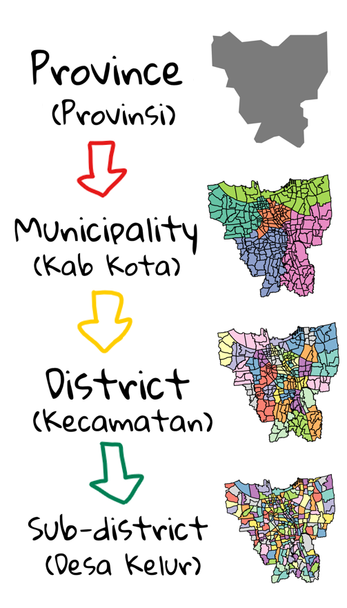
DKI Jarkarta is a province divided into municipalities (Kab Kota) which are further divided into districts (kecamatan) and finally divided into sub-districts (Desa Kelur)
3.2.2 Data Preprocessing
3.2.2.1 Invalid Geometries
length(which(st_is_valid(bd_jakarta) == FALSE))[1] 0Everything is valid
3.2.2.2 Exclude redundant fields
Exclude all data except Municipality, District name, District Code, Sub-district Code, Sub-district name, Total Population and geometry of the regions.
bd_jakarta <- bd_jakarta %>%
  select(2:4, 6:7, 9,)
3.2.2.3 Rename from Bahasa Indonesia to English
| Index | Original Name | Translated Name |
|---|---|---|
| 2 | KODE_DESA | Sub_District_Code |
| 3 | DESA | Sub_District |
| 4 | KODE | District_Code |
| 6 | KAB_KOTA | Municipality |
| 7 | KECAMATAN | District |
| 9 | JUMLAH_PEN | Total_Population |
Code
bd_jakarta <- bd_jakarta %>%
  dplyr::rename(
    Municipality=KAB_KOTA,
    District=KECAMATAN,
    District_Code=KODE,
    Sub_District=DESA,
    Sub_District_Code=KODE_DESA,
    Total_Population=JUMLAH_PEN
    )
3.2.2.4 Handle Missing Values
Code
cat("There are", sum(is.na(bd_jakarta)), "missing values in", paste(names(which(colSums(is.na(bd_jakarta))>0)), collapse = ", "))There are 4 missing values in Municipality, DistrictRemove all rows with missing values
bd_jakarta <- na.omit(bd_jakarta)3.2.3 Transform Coordinate System
st_crs(bd_jakarta)Coordinate Reference System:
User input: WGS 84
wkt:
GEOGCRS["WGS 84",
DATUM["World Geodetic System 1984",
ELLIPSOID["WGS 84",6378137,298.257223563,
LENGTHUNIT["metre",1]]],
PRIMEM["Greenwich",0,
ANGLEUNIT["degree",0.0174532925199433]],
CS[ellipsoidal,2],
AXIS["latitude",north,
ORDER[1],
ANGLEUNIT["degree",0.0174532925199433]],
AXIS["longitude",east,
ORDER[2],
ANGLEUNIT["degree",0.0174532925199433]],
ID["EPSG",4326]]Transform the CRS to DGN95, ESPG code 23845
bd_jakarta <- st_transform(bd_jakarta, 23845)st_crs(bd_jakarta)Coordinate Reference System:
User input: EPSG:23845
wkt:
PROJCRS["DGN95 / Indonesia TM-3 zone 54.1",
BASEGEOGCRS["DGN95",
DATUM["Datum Geodesi Nasional 1995",
ELLIPSOID["WGS 84",6378137,298.257223563,
LENGTHUNIT["metre",1]]],
PRIMEM["Greenwich",0,
ANGLEUNIT["degree",0.0174532925199433]],
ID["EPSG",4755]],
CONVERSION["Indonesia TM-3 zone 54.1",
METHOD["Transverse Mercator",
ID["EPSG",9807]],
PARAMETER["Latitude of natural origin",0,
ANGLEUNIT["degree",0.0174532925199433],
ID["EPSG",8801]],
PARAMETER["Longitude of natural origin",139.5,
ANGLEUNIT["degree",0.0174532925199433],
ID["EPSG",8802]],
PARAMETER["Scale factor at natural origin",0.9999,
SCALEUNIT["unity",1],
ID["EPSG",8805]],
PARAMETER["False easting",200000,
LENGTHUNIT["metre",1],
ID["EPSG",8806]],
PARAMETER["False northing",1500000,
LENGTHUNIT["metre",1],
ID["EPSG",8807]]],
CS[Cartesian,2],
AXIS["easting (X)",east,
ORDER[1],
LENGTHUNIT["metre",1]],
AXIS["northing (Y)",north,
ORDER[2],
LENGTHUNIT["metre",1]],
USAGE[
SCOPE["Cadastre."],
AREA["Indonesia - onshore east of 138°E."],
BBOX[-9.19,138,-1.49,141.01]],
ID["EPSG",23845]]3.2.4 Remove outer islands
Based on first glance in View, there are several small islands surrounding the mainland. As this is not relevant to the analysis, they shall be omitted.
# KEPULAUAN SERIBU means thousand islands
bd_jakarta <- filter(bd_jakarta, Municipality != "KEPULAUAN SERIBU")
3.2.5 Data Summary
Code
c = length(unique(bd_jakarta$"Municipality"))
d = length(unique(bd_jakarta$"District"))
sd = length(unique(bd_jakarta$"Sub_District"))

cat("There are", c, "unique municipalities,", d, "unique districts, and", sd, "unique sub-districs")
There are 5 unique municipalities, 42 unique districts, and 261 unique sub-districs3.2.5.1 View distribution
Code
df_grp_municipality = bd_jakarta %>% group_by(Municipality)  %>%
                    summarise(total_districts = n(),
                              .groups = 'drop')

ggplot(df_grp_municipality, aes(x=Municipality, y=total_districts), fill=Municipality) +
  geom_bar(stat = "identity",
           color="black",
           fill="lightblue4") +
  ggtitle("Number of Districts by Municipality") +
  xlab("Municipality Name") +
ylab("No. of Districts") 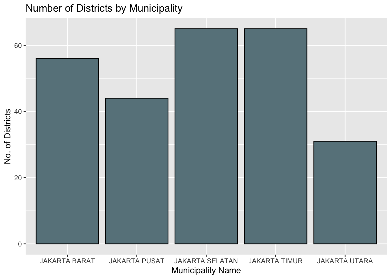
Code
df_grp_districs = bd_jakarta %>% group_by(District)  %>%
                    summarise(total_sub_districts = n(),
                              .groups = 'drop')

ggplot(df_grp_districs, aes(x=District, y=total_sub_districts)) +
  geom_bar(stat = "identity",
           color="black",
           fill="lightblue3") +
  scale_x_discrete(guide = guide_axis(n.dodge=7))+
  ggtitle("Number of Sub-districts by District") +
  xlab("District Name") +
ylab("No. of Sub-districts") 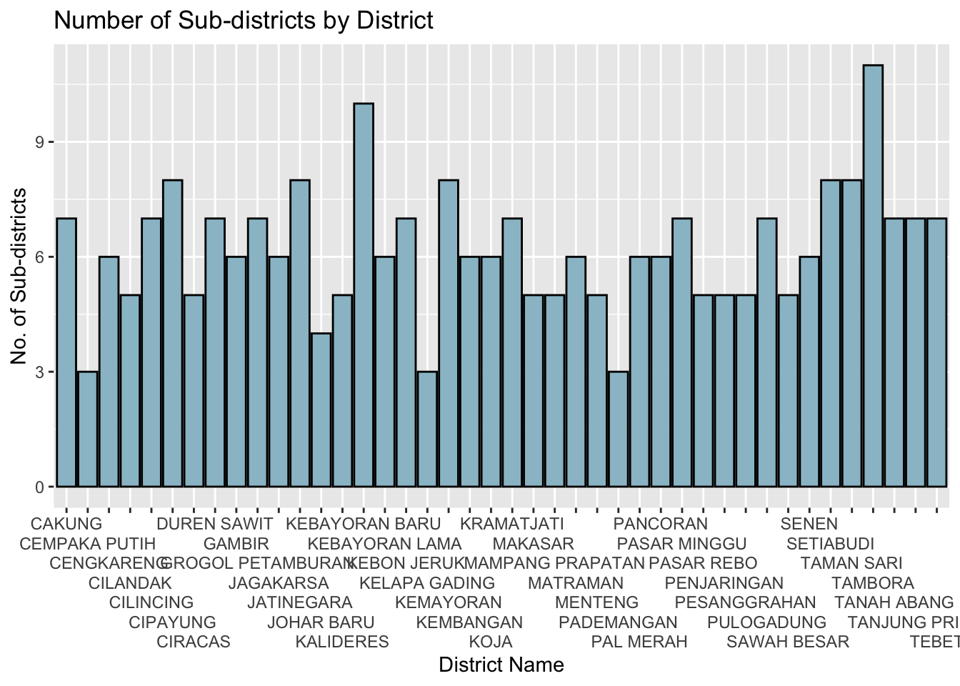
3.2.5.2 View by Municipality Divisions
tm_shape(bd_jakarta) +
  tm_polygons("Municipality")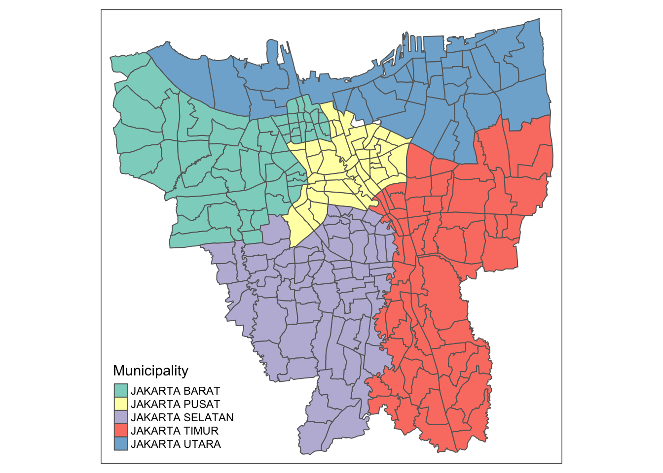
3.2.5.2 View by Population
ggplot(bd_jakarta, aes(x=Total_Population)) +
  geom_histogram(bins = 10,
                color="black",
                fill="indianred")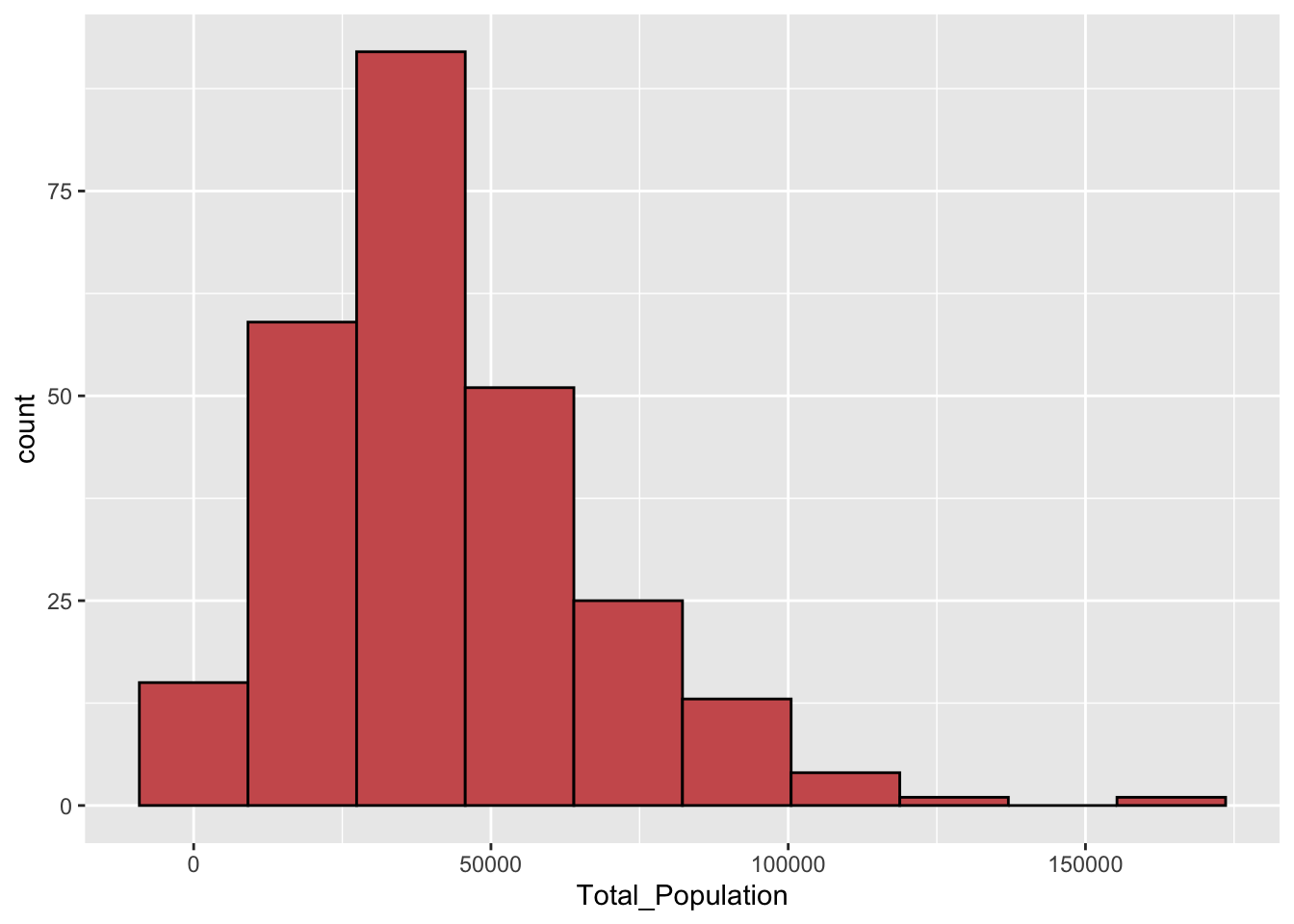
Equal Interval Classification
Code
tmap_mode("plot")
tm_shape(bd_jakarta) +
  tm_fill("Total_Population",
          style = "equal",
          palette = "OrRd") +
  tm_layout(main.title = "Distribution by Population") +
tm_borders(alpha = 0.5) 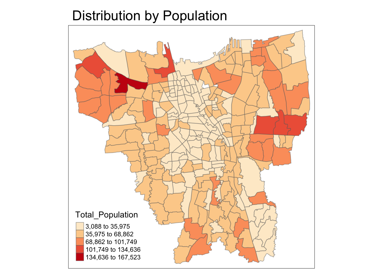
3.3 Aspatial Data
3.3.1 Load Data
All files were downloaded as “Data Vaksinasi Berbasis Kelurahan (<last date of month> <Indonesian month name> <year>).xlsx” were locally renamed as “<last date of month> <English month name> <year>.xlsx”
#get list of aspatial data files
folder_path <- "data/aspatial"
files <- list.files(folder_path, pattern = ".xlsx", full.names = TRUE)
There was no file for Feb 28, 2022 so vaccination rate as of Feb 27, 2022 has been used instead
#combines files into vacc_df
vacc_df <- data.frame()

for (file in files) {
  data <- read_excel(file, sheet = "Data Kelurahan") #sub-district
  data$Date <- dmy(str_extract(file, "\\d{2} [[:alpha:]]+ \\d{4}")) #add date column
  vacc_df <- bind_rows(vacc_df, data)
}
3.3.2 Data Preprocessing
3.3.2.1 Exclude redundant fields
Exclude all values except Municipality name, Sub-district name, Sub-district code, Target number, Number not yet vaccinated, Total vaccines administered and Date.
vacc_df <-  vacc_df %>%
  select(1:2, 4:6, 9, 28)
3.3.2.2 Rename from Bahasa Indonesia to English
| Index | Original Name | Translated Name |
|---|---|---|
| 1 | KODE KELURAHAN | Sub_District_Code |
| 2 | WILAYAH KOTA | Municipality |
| 4 | KELURAHAN | Sub_District |
| 5 | SANSARAN | Target |
| 6 | BELUM VAKSIN | Not_Yet_Vaccinated |
| 9 | TOTAL VAKSIN DIBERIKAN | Total_Vaccine_Administered |
Code
vacc_df <- vacc_df %>%
  dplyr::rename(
    Municipality="WILAYAH KOTA",
    Sub_District="KELURAHAN",
    Sub_District_Code="KODE KELURAHAN",
    Target="SASARAN",
    Not_Yet_Vaccinated="BELUM VAKSIN",
    Total_Vaccine_Administered="TOTAL VAKSIN\r\nDIBERIKAN"
    )
3.3.2.3 Handle Missing Values
Code
cat("There are", sum(is.na(vacc_df)), "missing values in", paste(names(which(colSums(is.na(vacc_df))>0)), collapse = ", "))There are 24 missing values in Sub_District_Code, MunicipalityRemove all rows with missing values
vacc_df <- na.omit(vacc_df)3.3.3 Remove outer islands
vacc_df <- filter(vacc_df, Municipality != "KAB.ADM.KEP.SERIBU")Remove column Municipality as there is no further need for it in this data frame
vacc_df = vacc_df[,!(names(vacc_df) %in% "Municipality")]3.4 Combined Data Wrangling
3.4.1 Join vaccination data
df <- left_join(bd_jakarta, vacc_df,
         by=c("Sub_District_Code"="Sub_District_Code",
              "Sub_District"="Sub_District"))
Visualise
Code
p1 = tm_shape(df)+
  tm_fill("Target") +
  tm_borders(alpha = 0.5) +
  tm_layout(main.title="Target")

p2 = tm_shape(df)+
  tm_fill("Total_Vaccine_Administered") +
  tm_borders(alpha = 0.5) +
  tm_layout(main.title="Total Vaccines Administered")


tmap_arrange(p1, p2)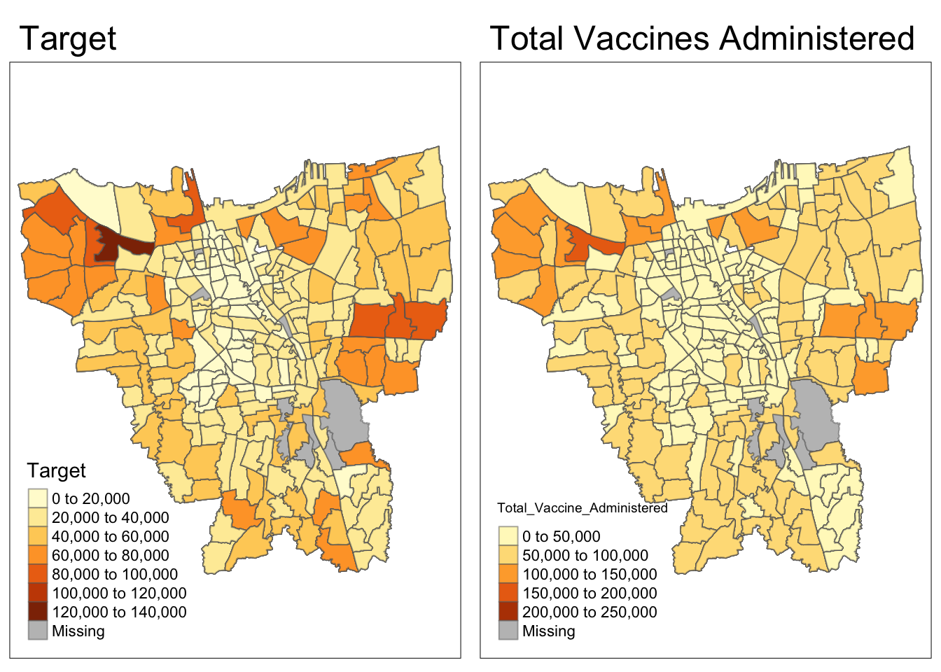
While Target and Total Vaccines Administered seem highly correlated, there several grey Missing patches which will be addressed below
3.4.2 Standardise Data
Although missing values from the geospatial and aspatial data have already been omitted, there is a “Missing” data in the above visualisation. This is because there are discrepancies between the sub-district names in the two datasets.
View Discrepancies
Code
cases_subdistrict <- c(vacc_df$Sub_District)
bd_subdistrict <- c(bd_jakarta$Sub_District)

aspatial_list <- sort(unique(cases_subdistrict[!(cases_subdistrict %in% bd_subdistrict)]))
aspatial_list <- c(aspatial_list[1:3], aspatial_list[6], aspatial_list[5], aspatial_list[7:9], aspatial_list[4]) #rearrgane - hardcoded

geospatial_list <- sort(unique(bd_subdistrict[!(bd_subdistrict %in% cases_subdistrict)]))


spelling <- data.frame(
  Aspatial_Cases=aspatial_list,
  Geospatial_BD=geospatial_list
  )

# with dataframe a input, outputs a kable
library(knitr)
library(kableExtra)
kable(spelling, caption="Mismatched Records") %>%
kable_material("hover", latex_options="scale_down")| Aspatial_Cases | Geospatial_BD |
|---|---|
| BALE KAMBANG | BALEKAMBANG |
| HALIM PERDANA KUSUMAH | HALIM PERDANA KUSUMA |
| JATI PULO | JATIPULO |
| KRAMAT JATI | KRAMATJATI |
| KERENDANG | KRENDANG |
| PAL MERIAM | PALMERIAM |
| PINANG RANTI | PINANGRANTI |
| RAWA JATI | RAWAJATI |
| KAMPUNG TENGAH | TENGAH |
Rename geospatial data with aspatial data values
for (i in 1:9) {
  bd_jakarta$Sub_District[bd_jakarta$Sub_District == geospatial_list[i]] <- aspatial_list[i]
}

rm(aspatial_list, geospatial_list, i) #cleanup
3.4.3 Join vaccination data (again)
df <- left_join(bd_jakarta, vacc_df,
        by=c("Sub_District_Code"="Sub_District_Code",
              "Sub_District"="Sub_District"))
Visualise
Code
p1 = tm_shape(df)+
  tm_fill("Target") +
  tm_borders(alpha = 0.5) +
  tm_layout(main.title="Target")

p2 = tm_shape(df)+
  tm_fill("Total_Vaccine_Administered") +
  tm_borders(alpha = 0.5) +
  tm_layout(main.title="Total Vaccines Administered")


tmap_arrange(p1, p2)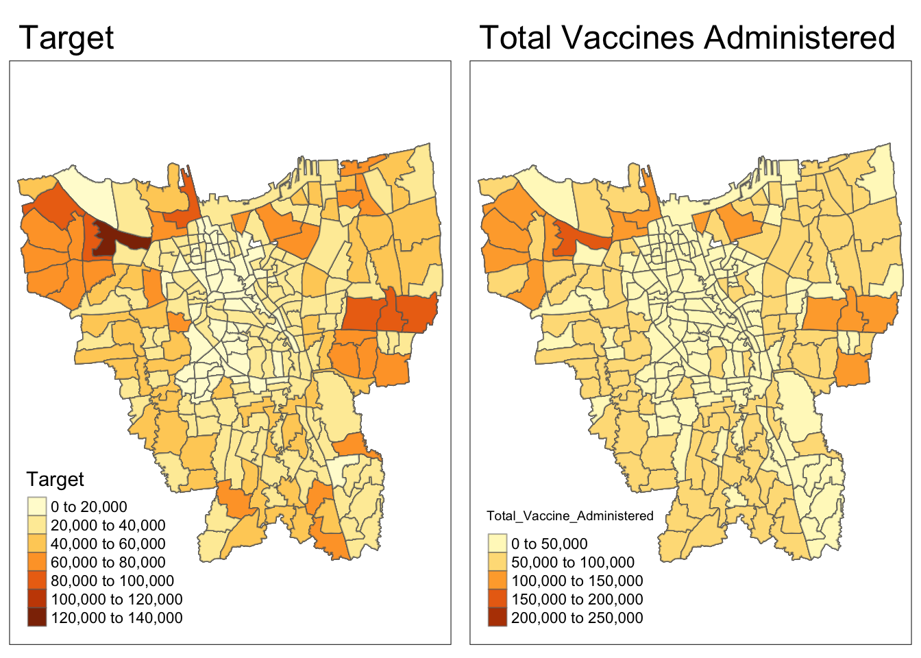
Grey Missing data from 3.4.1 has been handled.
4.0 Choropleth Mapping
4.1 Compute Vaccination Rates
\[ \mathrm Vaccination \ Rate = \frac{\mathrm Target \ - \ (\mathrm Not \ Vaccinated) \ }{\mathrm Target} \ * 100 \]
(Target has been chosen over total population to excluse people who are not required to be vaccinated)
Add Vaccination Rate column to main dataframe (df)
df <- df %>%
  mutate(vaccination_rate = ((Target-Not_Yet_Vaccinated)/Target)*100)
Create table vacc_rate_df that groups vaccination rate by sub-district and date
vacc_rate_df <- df %>%
  st_drop_geometry  %>% #remove geometry for pivot
  group_by(Sub_District, Date) %>%
  summarise(vaccination_rate) %>%

  ungroup() %>%
  pivot_wider(names_from = Date, #use pivot table to rearrange
              values_from = vaccination_rate) %>%

  left_join(bd_jakarta, by=c("Sub_District"="Sub_District")) #add geometry back
View
head(vacc_rate_df)# A tibble: 6 × 19
Sub_District 2021-07…¹ 2021-…² 2021-…³ 2021-…⁴ 2021-…⁵ 2021-…⁶ 2022-…⁷ 2022-…⁸
<chr> <dbl> <dbl> <dbl> <dbl> <dbl> <dbl> <dbl> <dbl>
1 ANCOL 48.5 61.6 72.1 75.0 76.9 78.9 80.6 80.8
2 ANGKE 52.8 64.6 74.2 77.7 79.6 80.9 81.7 81.9
3 BALE KAMBANG 37.0 57.0 70.0 73.9 76.6 78.2 79.5 79.7
4 BALI MESTER 47.0 62.0 74.2 78.2 80.3 81.7 82.8 83.1
5 BAMBU APUS 47.6 64.2 76.2 80.9 82.5 83.4 84.5 84.7
6 BANGKA 51.6 61.3 73.2 78.0 79.8 80.7 81.5 81.7
# … with 10 more variables: `2022-03-31` <dbl>, `2022-04-30` <dbl>,
# `2022-05-31` <dbl>, `2022-06-30` <dbl>, Sub_District_Code <chr>,
# District_Code <dbl>, Municipality <chr>, District <chr>,
# Total_Population <dbl>, geometry <MULTIPOLYGON [m]>, and abbreviated
# variable names ¹`2021-07-31`, ²`2021-08-31`, ³`2021-09-30`, ⁴`2021-10-31`,
# ⁵`2021-11-30`, ⁶`2021-12-31`, ⁷`2022-01-31`, ⁸`2022-02-27`Convert to sf object for plotting
vacc_rate_df <- st_as_sf(vacc_rate_df)4.2 Visualise monthly vaccination rates
Code
#helper function for plots
#Can use fisher too


plot <- function(varname) {
  tm_shape(vacc_rate_df) +
    tm_polygons() +
  tm_shape(vacc_rate_df) +
    tm_fill(varname,
          n= 6,
          style = "jenks",
          palette="RdPu",
          title = "Vaccination Rate (%)") +
    tm_layout(main.title = paste("Vaccination rate by", paste(month(ymd(varname), label=TRUE), year(ymd(varname)))),
          main.title.position = "center",
          frame = TRUE) +
    tm_borders(alpha = 0.5)
}
Plot
Code
tmap_mode("plot")
tmap_arrange(plot("2021-07-31"), plot("2021-08-31"), plot("2021-09-30"),plot("2021-10-31"))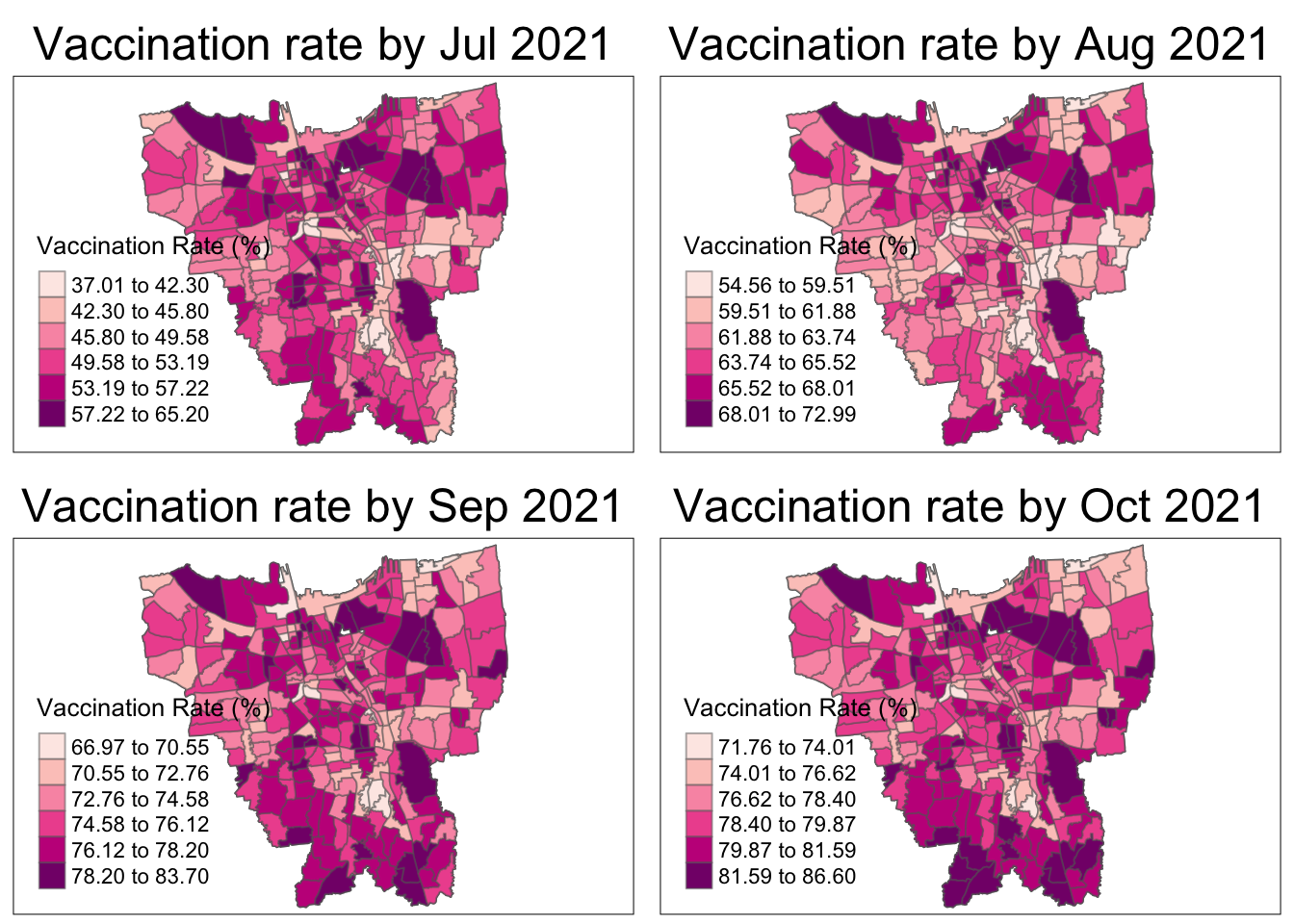
Code
tmap_mode("plot")
tmap_arrange(plot("2021-11-30"), plot("2021-12-31"), plot("2022-01-31"), plot("2022-02-27"))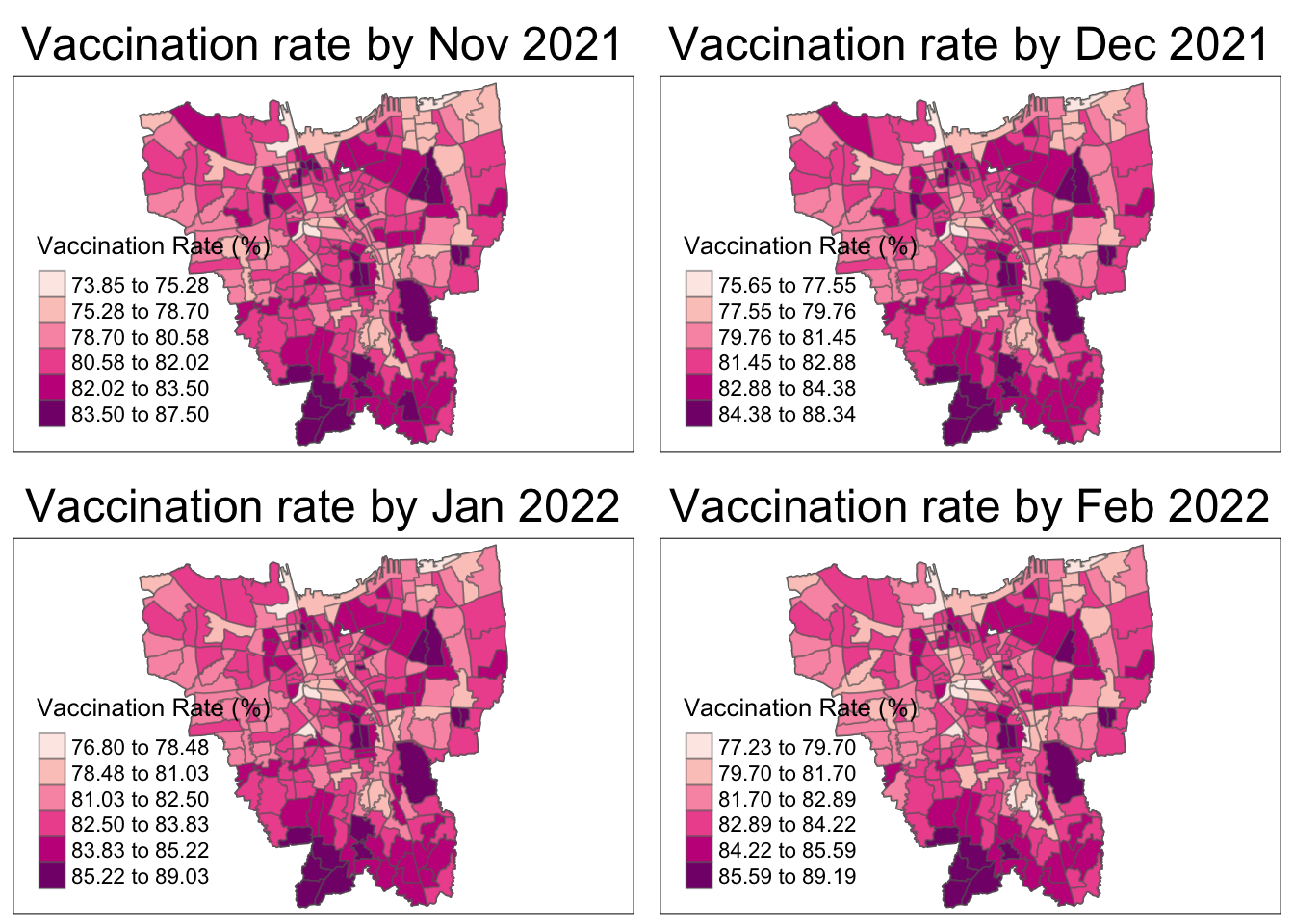
Code
tmap_mode("plot")
tmap_arrange(plot("2022-03-31"), plot("2022-04-30"), plot("2022-05-31"), plot("2022-06-30"))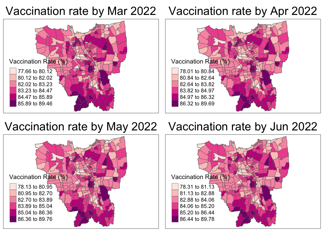
The vaccination rate increases over the year for all regions. The Northern municipality starts with the highest vaccination rates then other regions, particularly the South and East, catch up.
4.3 Observations from Jenks based Mapping
4.3.1 Vaccination Rates by Sub-district
For lowest vaccination rates,
Code
#temporary dataset
temp_low <- df %>%
  group_by(Date) %>%
  filter(vaccination_rate == min(vaccination_rate)) %>%
  arrange(Date)

#plot
ggplotly(ggplot(temp_low, aes(x=Date, y=vaccination_rate)) +
  geom_point(aes(color=temp_low$Sub_District)) +
  ggtitle("Lowest Vaccination Rates over the Year by Sub-district"))
Not only does the minimum vaccination rate increase over year, but the sub-district Bale Kambang has a sharp increase in its rate and no longer has the lowest vaccination rate by July 2022.
For highest vaccination rates,
Code
#temporary dataset
temp_high <- df %>%
  group_by(Date) %>%
  filter(vaccination_rate == max(vaccination_rate)) %>%
  arrange(Date)

#plot
ggplotly(ggplot(temp_high, aes(x=Date, y=vaccination_rate)) +
  geom_point(aes(color=temp_high$Sub_District)) +
  ggtitle("Highest Vaccination Rates over the Year by Sub-district"))
The sub-district Halim Perdana Kusumah has the highest vaccination rate for the most part.
The vaccination rate by July 31, 2021 for this sub-district at 65.21% is much higher than that of Bale Kambang which was at 37.01%. This difference of 28.20% gets smoothed down to 11.47% by June 30, 2022.
temp <- data.frame(temp_low$Date, temp_low$vaccination_rate, temp_high$vaccination_rate)

colors <- c("Lowest" = "orange", "Highest" = "steelblue")

ggplotly(ggplot(temp, aes(x=temp_low.Date)) +
  geom_line(aes(y=temp_low.vaccination_rate, color="Lowest"), size = 1.2) +
  geom_line(aes(y=temp_high.vaccination_rate, color="Highest"), size = 1.2) +
  ggtitle("Highest and Lowest Vaccination Rates over the Year by Sub-district") +
  labs(y = "Vaccination Rate (%)",
      color = "Vaccination Rate") +
  scale_color_manual(values = colors))
4.3.2 Spatio-Temporal Mapping with custom breakpoints
View how the vaccination rate increases in all regions over the year based on Jenks defined breakpoints.
With the lowest and highest vaccination rates over the year being 37% and 90%, the Jenks breakpoints are defined as follows
breakpoints = c(37, 55, 72, 80, 84, 90)Code
#helper function for plotting
plot <- function(varname) {
  tm_shape(vacc_rate_df) +
    tm_polygons() +
  tm_shape(vacc_rate_df) +
    tm_fill(varname,
          breaks= breakpoints,
          palette="RdPu",
          title = "Vaccination Rate") +
    tm_layout(main.title = paste("Vaccination rate by", paste(month(ymd(varname), label=TRUE), year(ymd(varname)))),
          main.title.position = "center",
          frame = TRUE) +
    tm_borders(alpha = 0.5)
}
Plot
Code
tmap_mode("plot")
tmap_arrange(plot("2021-07-31"), plot("2021-08-31"), plot("2021-09-30"),plot("2021-10-31"))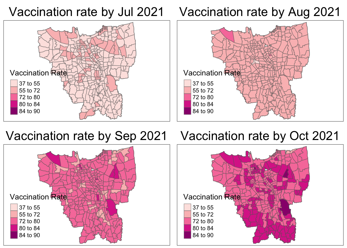
Code
tmap_mode("plot")
tmap_arrange(plot("2021-11-30"), plot("2021-12-31"), plot("2022-01-31"), plot("2022-02-27"))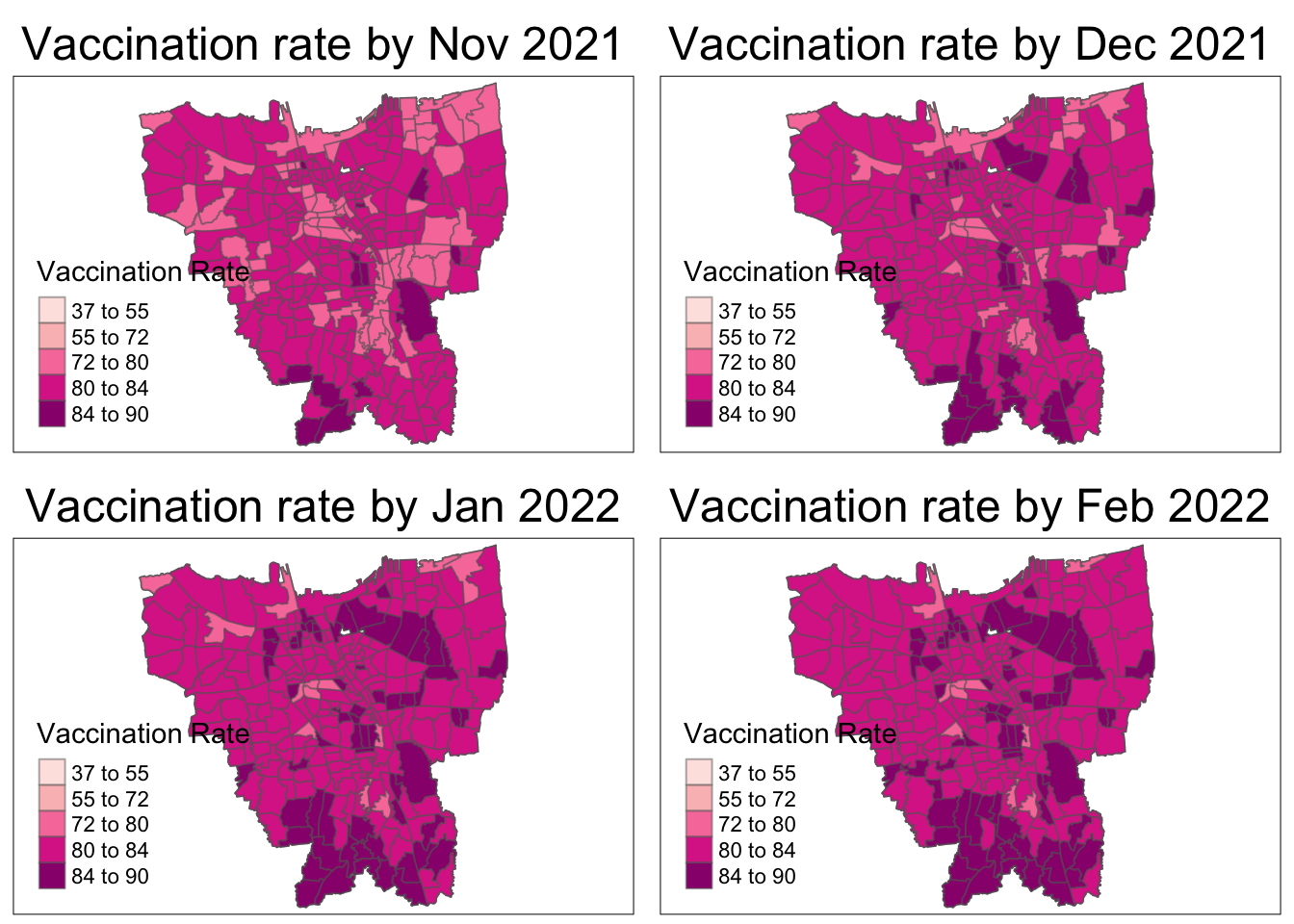
Code
tmap_mode("plot")
tmap_arrange(plot("2022-03-31"), plot("2022-04-30"), plot("2022-05-31"), plot("2022-06-30"))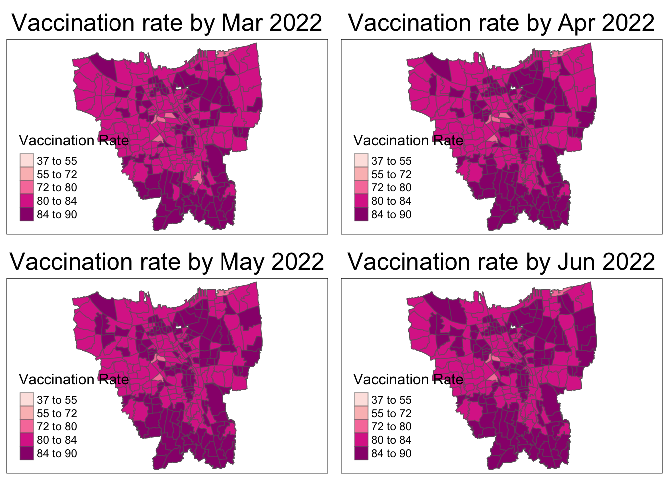
As aforementioned, the overall vaccination rates grew from July 2021, to June 2022. From the maps, it is observed that the rates grew quickly till December 2021 and then grew at a steady pace.
In July 2021, there is a slightly higher vaccination rate in the North and Western municipalities which quickly becomes uniform by August 2021.
From October 2021, it is seems that the Northern and Southern municipalities have the higher vaccination rates than their surrounding regions. The Eastern municipality catches up the fastest by March 2022 and the rest gradually catch up by June 2022.
5.0 Local Gi* Analysis
5.1 Compute Gi* values
5.1.1. Create attribute table
# make table with Date, Sub_District, Target, Not_Yet_Vaccinated
vacc_attr_table <- df %>% select(10, 8, 7, 2) %>% st_drop_geometry()

# add a new field for Vaccination_Rate
vacc_attr_table$Vaccination_Rate <- (vacc_attr_table$Target - vacc_attr_table$Not_Yet_Vaccinated) / vacc_attr_table$Target*100

# final vaccination attribute table with Date, Sub_District, Vaccination_Rate
vacc_attr_table <- tibble(vacc_attr_table %>% select(1,4,5))
5.1.2 Create a time series cube (spatio-temporal cube)
vacc_rate_st <- spacetime(vacc_attr_table, bd_jakarta,
                          .loc_col = "Sub_District",
                          .time_col = "Date")

#check valid
is_spacetime_cube(vacc_rate_st)
[1] TRUE5.1.3 Derive spatial weights
vacc_rate_nb <- vacc_rate_st %>%
  activate("geometry") %>%
         #neighbours
  mutate(nb = include_self(st_contiguity(geometry)),
         #inverse distance weights
         wt = st_inverse_distance(nb, geometry,
                                  scale=1,
                                  alpha=1),
         .before=1) %>%
  set_nbs("nb") %>%
  set_wts("wt")
View
head(vacc_rate_nb)# A tibble: 6 × 5
Date Sub_District Vaccination_Rate nb wt
<date> <chr> <dbl> <list> <list>
1 2021-07-31 KEAGUNGAN 53.3 <int [6]> <dbl [6]>
2 2021-07-31 GLODOK 61.6 <int [7]> <dbl [7]>
3 2021-07-31 HARAPAN MULIA 49.7 <int [6]> <dbl [6]>
4 2021-07-31 CEMPAKA BARU 46.7 <int [7]> <dbl [7]>
5 2021-07-31 PASAR BARU 59.3 <int [9]> <dbl [9]>
6 2021-07-31 KARANG ANYAR 52.2 <int [7]> <dbl [7]>5.1.4 Compute Gi* values
Set Seed for replicable results
set.seed(1234)Compute
#LISA
gi_val <- vacc_rate_nb |>
  group_by(Date) |>
  mutate(gi_val = local_gstar_perm(
    Vaccination_Rate, nb, wt, nsim=99)) |>
      tidyr::unnest(gi_val)
View
colnames(gi_val) [1] "Date" "Sub_District" "Vaccination_Rate" "nb"
[5] "wt" "gi_star" "e_gi" "var_gi"
[9] "p_value" "p_sim" "p_folded_sim" "skewness"
[13] "kurtosis" head(gi_val)# A tibble: 6 × 13
# Groups: Date [1]
Date Sub_Dis…¹ Vacci…² nb wt gi_star e_gi var_gi p_value p_sim
<date> <chr> <dbl> <lis> <lis> <dbl> <dbl> <dbl> <dbl> <dbl>
1 2021-07-31 KEAGUNGAN 53.3 <int> <dbl> 2.44 0.00383 2.13e-8 1.46e-2 0.02
2 2021-07-31 GLODOK 61.6 <int> <dbl> 3.85 0.00384 1.56e-8 1.18e-4 0.02
3 2021-07-31 HARAPAN … 49.7 <int> <dbl> 0.309 0.00382 2.20e-8 7.57e-1 0.84
4 2021-07-31 CEMPAKA … 46.7 <int> <dbl> -1.05 0.00383 1.53e-8 2.96e-1 0.34
5 2021-07-31 PASAR BA… 59.3 <int> <dbl> 2.71 0.00383 1.38e-8 6.82e-3 0.02
6 2021-07-31 KARANG A… 52.2 <int> <dbl> 1.67 0.00382 2.17e-8 9.49e-2 0.1
# … with 3 more variables: p_folded_sim <dbl>, skewness <dbl>, kurtosis <dbl>,
# and abbreviated variable names ¹Sub_District, ²Vaccination_Rate5.2 Visualise Gi* maps of the monthly vaccination rate
Combine Gi* values to main df
gi_val_df <- df %>%
  left_join(gi_val,
            by = c("Sub_District", "Date"))
Visualising Gi* and p-value of Gi* for significant locations (p-value < 0.05)
Code
#helper function for plotting
plot <- function(varname){
 gi_plot <-
    tm_shape(filter(gi_val_df, Date == varname)) +
    tm_polygons() +
    tm_shape(gi_val_df %>% filter(p_sim <0.05)) +
    tm_fill("gi_star",
            style="equal",
            n=5,
            palette = "seq") +
    tm_borders(alpha = 0.5) +
    tm_layout(main.title = paste("Significant Local Gi for", paste(month(ymd(varname), label=TRUE), year(ymd(varname)))),
              main.title.size = 0.8,
              aes.palette = list(seq = "-RdBu"))
  return(gi_plot)
}
Code
tmap_mode("plot")
tmap_arrange(plot("2021-07-31"), plot("2021-08-31"), plot("2021-09-30"),plot("2021-10-31"))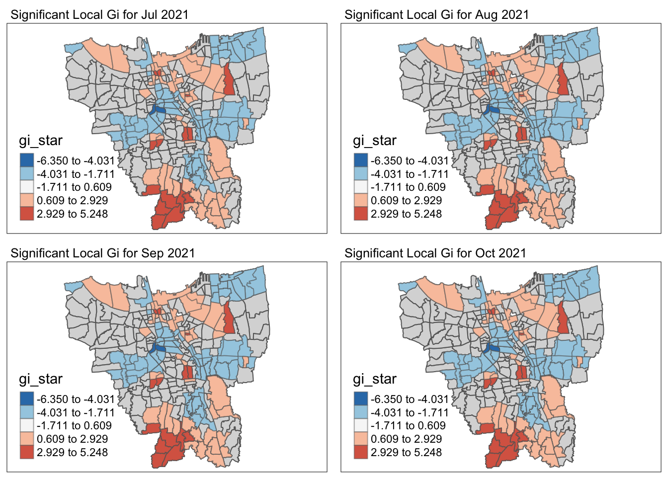
Code
tmap_mode("plot")
tmap_arrange(plot("2021-11-30"), plot("2021-12-31"), plot("2022-01-31"), plot("2022-02-27"))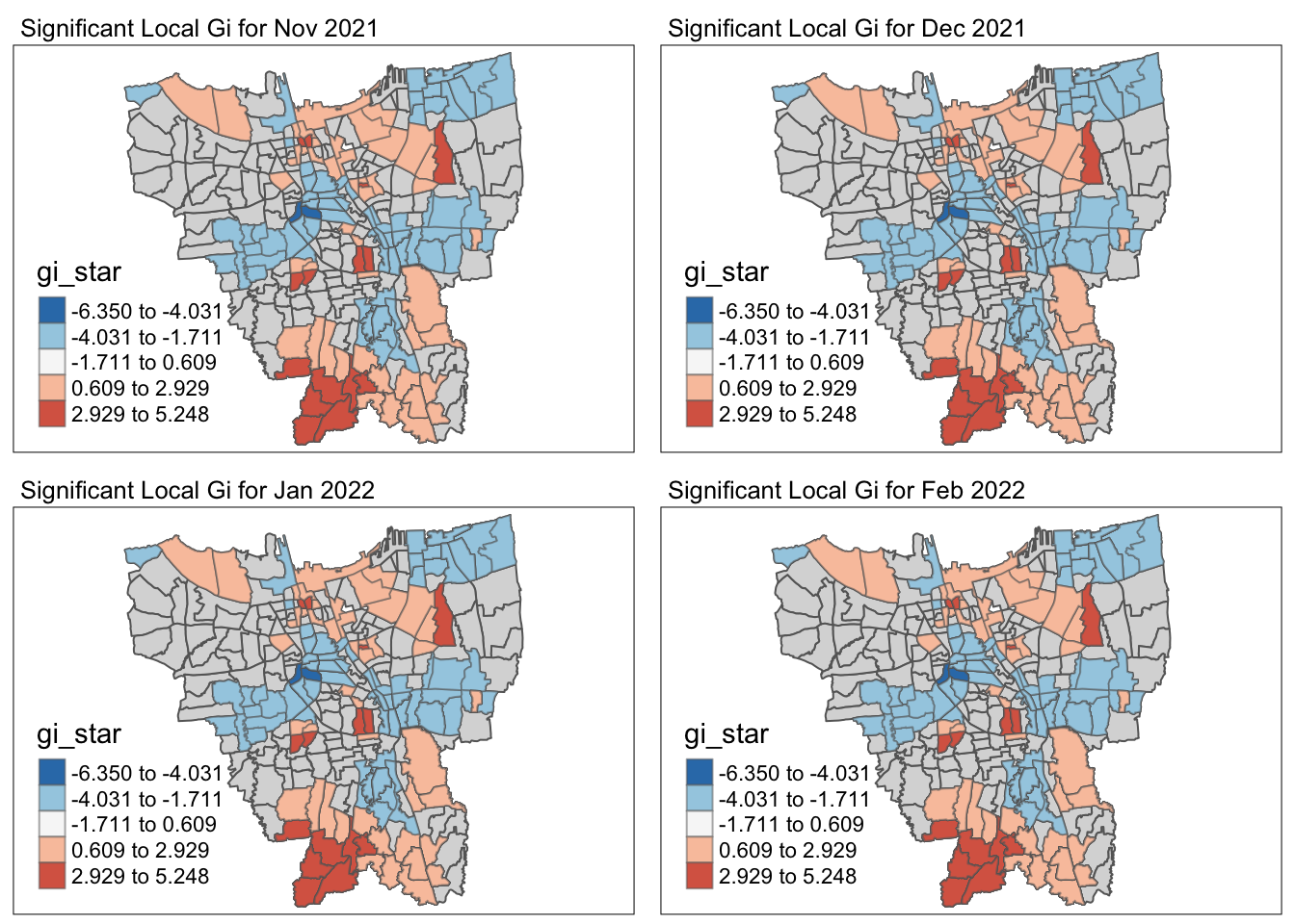
Code
tmap_mode("plot")
tmap_arrange(plot("2022-03-31"), plot("2022-04-30"), plot("2022-05-31"), plot("2022-06-30"))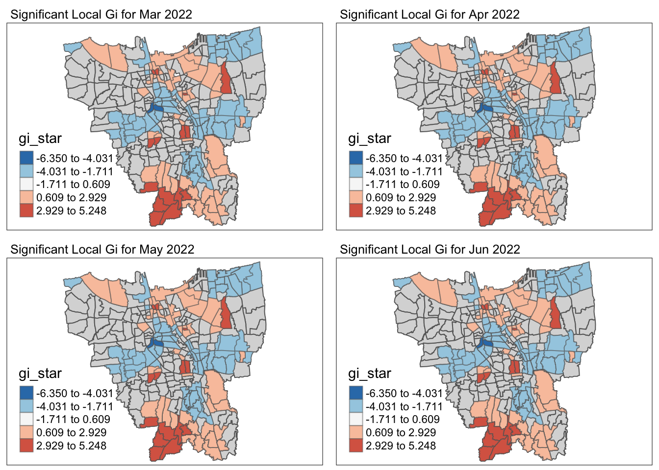
5.3 Observations of the Local Gi* Analysis
Filter by significant p-value (<0.05)
p_value_freq = filter(gi_val_df, p_sim<0.05)
temp <- as.data.frame(table(p_value_freq$Sub_District))
Code
cat("Throughout the 12 months, there were", nrow(temp), "Sub-districts with p-value of Gi* < 0.05 for at least 1 month")Throughout the 12 months, there were 128 Sub-districts with p-value of Gi* < 0.05 for at least 1 monthCode
cat("The Gi* value of the vaccination rates for the entire time period were significantly low / high for the", nrow(temp %>% filter(Freq == 12)), "following Sub-districts throughout the year - ")The Gi* value of the vaccination rates for the entire time period were significantly low / high for the 10 following Sub-districts throughout the year - | Sub-District | Municipality | Significance |
|---|---|---|
| BATU AMPAR | East | Low |
| CIPINANG CEMPEDAK | East | Low |
| GLODOK | West | High |
| KAMPUNG BALI | Central | Low |
| KAMPUNG TENGAH | East | Low |
| KEAGUNGAN | West | High |
| KEBON KACANG | Central | Low |
| KEBON MELATI | Central | Low |
| MANGGA BESAR | West | High |
| PETAMBURAN | Central | Low |
It is observed the Central and Eastern municipalities have very distributed vaccination rates throughout the year whereas the Western municipality has evenly distributed vaccinated rates throughout the year.
6.0 Emerging Hot Spot Analysis (EHSA)
6.1 Mann-Kendall Test
Perform the Mann-Kendall Test using the spatio-temporal local Gi* values on the following Sub-districts - “ANCOL”,“KOJA” and “JOHAR BARU”
sub_list = list("KAMAL","KOJA", "ANCOL")Filter data
cbg <- gi_val %>%
  ungroup() %>%
  filter(Sub_District %in% sub_list) |>
select(Date, Sub_District, gi_star)Plot
Code
cbg_ <-filter(cbg, Sub_District==sub_list[1])

ggplotly(ggplot(data=cbg_, aes(x=Date, y=gi_star))+
    geom_line()+
    theme_light())
P-value of Mann-Kendall Test
cbg_ |>
  summarise(mk = list(
    unclass(
      Kendall::MannKendall(gi_star)))) |>
  tidyr::unnest_wider(mk)
# A tibble: 1 × 5
tau sl S D varS
<dbl> <dbl> <dbl> <dbl> <dbl>
1 -0.848 0.000162 -56 66.0 213.The p-value (sl) is 0.0002 which is < 0.05 hence p-value is significant and tau is -0.85 This means there is an overall significant downward trend.
Plot
Code
cbg_ <-filter(cbg, Sub_District==sub_list[2])

ggplotly(ggplot(data=cbg_, aes(x=Date, y=gi_star))+
    geom_line()+
    theme_light())
P-value of Mann-Kendall Test
cbg_ |>
  summarise(mk = list(
    unclass(
      Kendall::MannKendall(gi_star)))) |>
  tidyr::unnest_wider(mk)
# A tibble: 1 × 5
tau sl S D varS
<dbl> <dbl> <dbl> <dbl> <dbl>
1 0.364 0.115 24 66.0 213.The p-value (sl) is 0.6 which is > 0.05 hence p-value is significant and tau is 0.21 This means there is an overall insignificant upward trend. This is because the Gi* values initially went down and then rose.
Plot
Code
cbg_ <-filter(cbg, Sub_District==sub_list[3])

ggplotly(ggplot(data=cbg_, aes(x=Date, y=gi_star))+
    geom_line()+
    theme_light())
P-value of Mann-Kendall Test
cbg_ |>
  summarise(mk = list(
    unclass(
      Kendall::MannKendall(gi_star)))) |>
  tidyr::unnest_wider(mk)
# A tibble: 1 × 5
tau sl S D varS
<dbl> <dbl> <dbl> <dbl> <dbl>
1 -0.273 0.244 -18 66.0 213.The p-value is 0.24 which is < 0.05 hence p-value is significant and tau is -0.27. This means there is an overall significant downward trend.
6.2 EHSA map of the Gi* values of the vaccination rate
6.2.1. Perform the Mann Kendall Test for each location
ehsa <- gi_val %>%
  group_by(Sub_District) %>%
  summarise(mk = list(
    unclass(
      Kendall::MannKendall(gi_star)))) %>%
  tidyr::unnest_wider(mk)
6.2.2. Arrange to show significant emerging hot/cold spots
emerging <- ehsa %>%
  arrange(sl, abs(tau)) %>%
  slice(1:5)
emerging
# A tibble: 5 × 6
Sub_District tau sl S D varS
<chr> <dbl> <dbl> <dbl> <dbl> <dbl>
1 PETOJO UTARA -0.970 0.0000156 -64 66.0 213.
2 KAYU MANIS 0.970 0.0000156 64 66.0 213.
3 JATINEGARA KAUM 0.939 0.0000287 62 66.0 213.
4 PISANGAN BARU 0.939 0.0000287 62 66.0 213.
5 PASAR BARU -0.939 0.0000288 -62 66.0 213.6.2.3. Performing Emerging Hotspot Analysis (EHSA)
ehsa <- emerging_hotspot_analysis(
  x = vacc_rate_st, #spacetime object
  .var = "Vaccination_Rate",
  k = 1, #number of time lags
  nsim = 99
)
Plot
Code
ggplot(data = ehsa,
       aes(x=classification, fill=classification, stat = "identity")) +
    scale_fill_manual(values=c("#8DD3C7", "#FFFFB3", "#BEBADA", "#FB8072")) +
    geom_bar()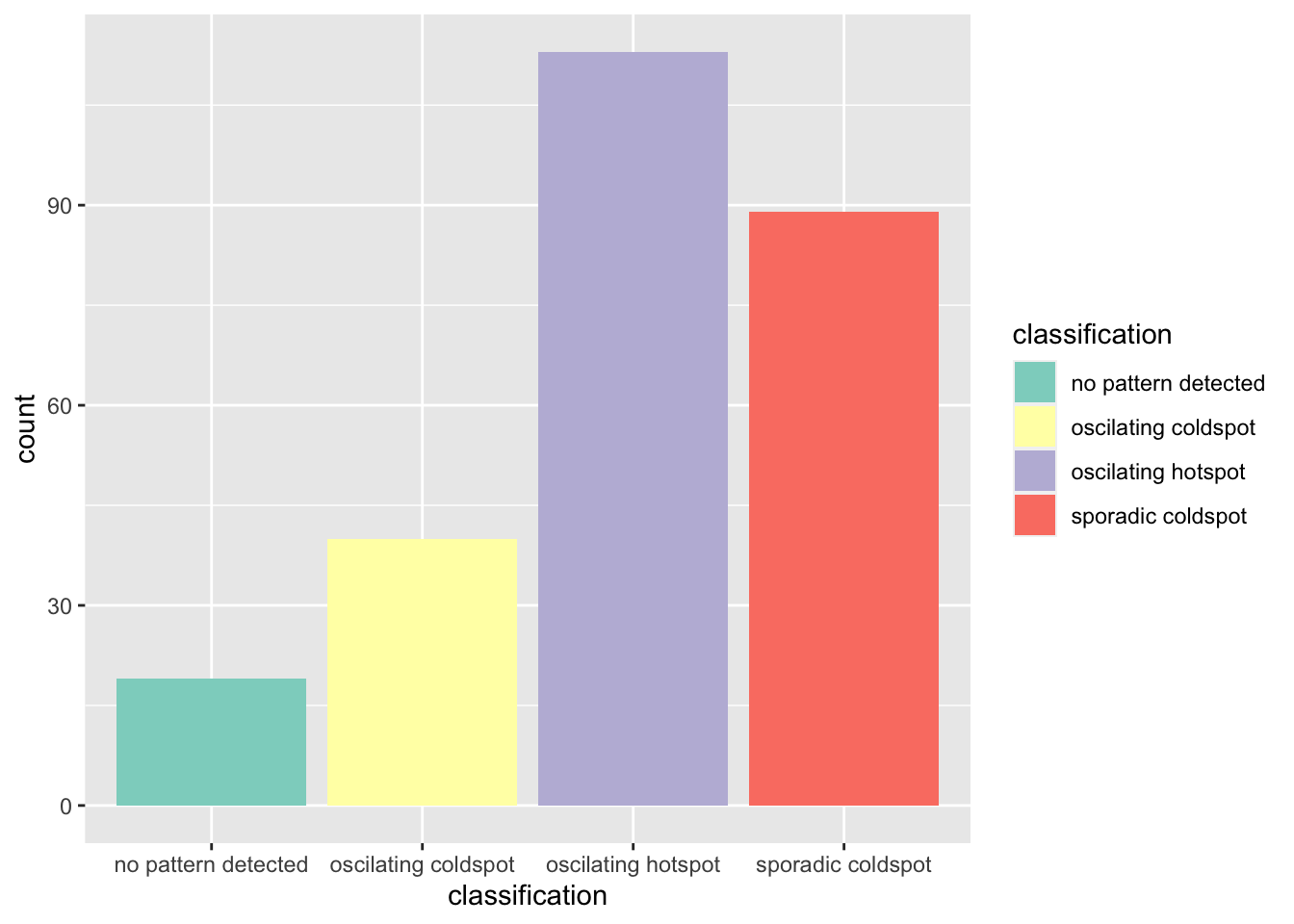
Oscillating hotspot class has the highest number of Sub-districts.
Combine EHSA values to main df nad add classification column
ehsa_df <- df %>%
  left_join(ehsa, by = c("Sub_District" = "location")) %>%
  mutate(NewClassification = case_when(p_value < 0.05 ~ classification,
                                       p_value >= 0.05 ~ "insignificant"))
Visualise
Code
tmap_mode("plot")
tm_shape(ehsa_df) +
  tm_polygons() +
  tm_borders(alpha = 0.5) +
tm_shape(ehsa_df %>% filter(NewClassification != "insignificant")) +
  tm_fill("NewClassification") +
  tm_borders(alpha = 0.4)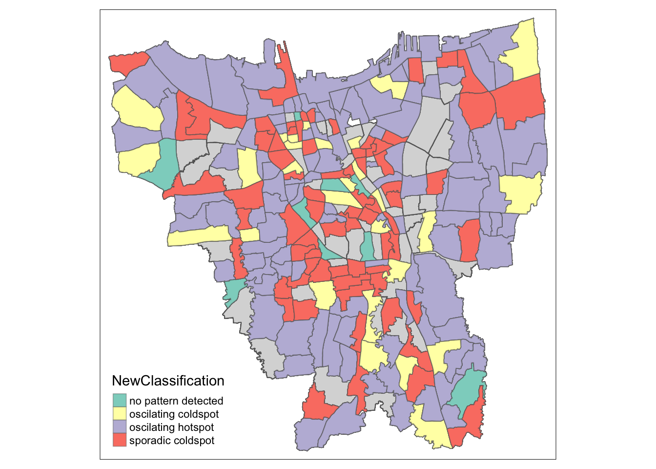
6.3 Observations of the spatial patterns
As aforementioned, most the places are categorised under oscillating hotspots. These points are evenly spread out throughout the province. This is because more sub-districts had higher vaccination rates over time.
The second most number of places, under sporadic coldspots seem to be more clustered towards the Central municipality. This is because that region had the lowest relative vaccination rates, despite increasing over the year.
Oscillating coldspots are evenly spread out throughout the province, more so towards the provincial borders. This is because those regions started with the highest vaccination rates but were relatively less than its neighbours over time.
Finally, with the fewest classes, the places where no patterns are detected seem to be mainly in the Central municipality.
7.0 Acknowledgements
I’d like to thank Professor Kam for his insights and resource materials provided under IS415 Geospatial Analytics and Applications.