Take Home Exercise 3

Published

March 22, 2023

Modified

March 26, 2023

1.0 Overview

1.1 Background

Housing is an essential component of household wealth worldwide. Buying a housing has always been a major investment for most people. The price of housing is affected by many factors. Some of them are global in nature such as the general economy of a country or inflation rate. Others can be more specific to the properties themselves. These factors can be further divided to structural and locational factors. Structural factors are variables related to the property themselves such as the size, fitting, and tenure of the property. Locational factors are variables related to the neighbourhood of the properties such as proximity to childcare centre, public transport service and shopping centre.

Conventional, housing resale prices predictive models were built by using Ordinary Least Square (OLS) method. However, this method failed to take into consideration that spatial autocorrelation and spatial heterogeneity exist in geographic data sets such as housing transactions. With the existence of spatial autocorrelation, the OLS estimation of predictive housing resale pricing models could lead to biased, inconsistent, or inefficient results (Anselin 1998). In view of this limitation, Geographical Weighted Models were introduced for calibrating predictive model for housing resale prices.

1.2 Task

In this take-home exercise, you are tasked to predict HDB resale prices at the sub-market level (i.e. HDB 3-room, HDB 4-room and HDB 5-room) for the month of January and February 2023 in Singapore. The predictive models must be built by using by using conventional OLS method and GWR methods. You are also required to compare the performance of the conventional OLS method versus the geographical weighted methods.

2.0 Setup

2.1 Import Packages

sf, spdep, sfdep - Used for handling geospatial data
tmap, plotly, ggplot2, corrplot - Used for visualizing dataframes and plots
units, maxtrixStats - Used for computing proximity matrix
ggpubr, olsrr, GWmodel, SpatialML - Used for model creation
Metrics - Used for calculating rmse
tidyVerse - Used for data transformation and presentation
onemapsgapi, httr, rjson - Used for data collection and wrangling

pacman::p_load(olsrr, corrplot, sf, spdep, tmap, tidyverse, sfdep, onemapsgapi, httr, rjson, plotly, ggplot2, units, matrixStats, heatmaply, ggpubr, Metrics, GWmodel, SpatialML)

3.0 Data Wrangling

3.1 Datasets Used

Type	Name
Aspatial	HDB Resale Data
Geospatial	Singapore Subzones (base layer)
Geospatial (factor)	Bus Stops
Geospatial (factor)	MRT Station Exits
Geospatial (factor)	Kindergartens
Geospatial (factor)	Childcare
Geospatial (factor)	Primary Schools
Geospatial (factor)	Sports Facilities
Geospatial (factor)	Parks
Geospatial (factor)	Gyms
Geospatial (factor)	Water Sites
Geospatial (factor)	Hawker Centers
Geospatial (factor)	Supermarkets
Geospatial (factor)	Eldercare
Geospatial (factor)	Waste Disposal
Geospatial (factor)	Active Cemeteries
Geospatial (factor)	Historic Sites

3.2 Aspatial Data

resale <- read_csv("data/aspatial/resale-flat-prices-based-on-registration-date-from-jan-2017-onwards.csv")

glimpse(resale)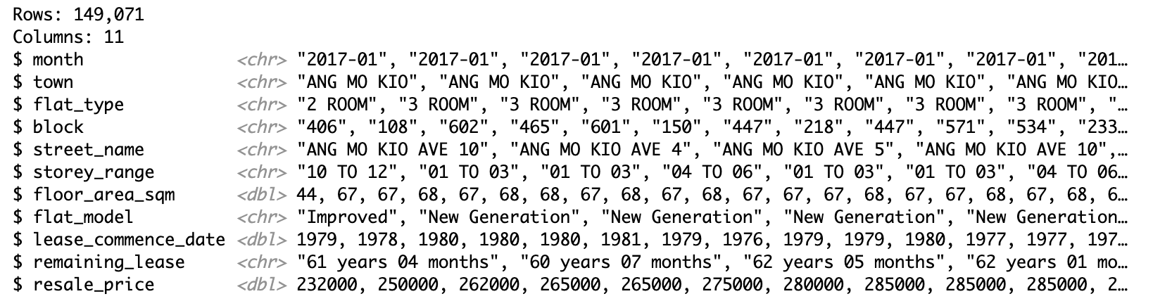

The dataset is based on the period of Jan 2017 to March 2023. It contains 11 columns with 149,071 rows.

3.2.2 Filter Data

The flat type has a high significance (p-value) of 2e-16 at 95% confidence level. This would impact the significance of all the other variables so the data is to be further split.

summary(aov(resale_price ~ flat_type, data = resale))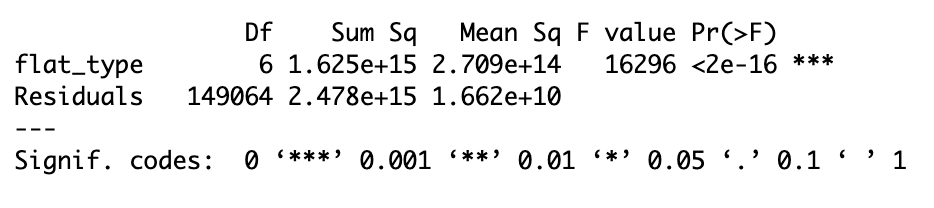

This exercise will use four bedroom flats only and for a shorter time period - Jan 01 2021 to Dec 31 2022 for train data and Jan 01 2023 to Feb 28 2023 for test data.

Filter
Glimpse

resale <- resale %>% 
  filter(flat_type == "3 ROOM") %>%
  filter(month >= "2021-01" & month <= "2022-12" | month >= "2023-01" & month <= "2023-02") %>%
  select(-c(town, flat_type, flat_model, lease_commence_date))  #drop irrelevant variables

Code

c = 13778 #nrow(resale)
cat("The dataset now contains", c, "rows.")

The dataset now contains 13778 rows.

3.2.3 Clean Up Variables

3.2.3.1 Street Address

Extract full address with joint block and street name. This will later be used to get the corresponding latitude and longitude of the addresses.

resale <- resale %>%
  mutate(resale, address = paste(block,street_name)) %>%
  select(-c(block, street_name)) #drop irrelevant variables

3.2.3.2 Remaining Lease

Extract numeric value of remaining lease from text

Code

str_list <- str_split(resale$remaining_lease, " ")
c = 1 #index counter

for(i in str_list) {
  year <- as.numeric(i[1])
  month = 0
  if(length(i) > 2) { #x years y months
    month <- as.numeric(i[3])
  }
  resale$remaining_lease[c] <- (year + round(month/12, 2))
  c = c + 1
}

resale<- resale |> 
  mutate(remaining_lease=as.numeric(remaining_lease))

3.2.3.3 Floor Level

The storey_range is a categorical variable with 15 categories - “01 TO 03”, “04 TO 06” upto “46 TO 48”. Keeping them as separate categories would induce high carnality into the model.

The distribution of the storey_range is as follows -

Code

ggplot(resale, aes(x= storey_range)) +
  geom_bar() +
  scale_x_discrete(guide = guide_axis(n.dodge=2))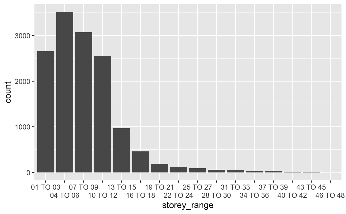

For ease of use and to lower the carnality, the data will be categorised into 3 divisions - 1,2,3 which would correspond to storeys 01-06, 07-12 and 13-48

Code

#get ordinal data of storey_range
storey_text <- unique(resale$storey_range)
storey_cat <- c(1,1,2,2, rep(3, 11))

#set label
resale$storey_num <- storey_cat[match(resale$storey_range, storey_text)] 
levels(resale$storey_num) <- storey_text

#change column to categorical data type
resale<- resale |> 
  mutate(storey_num=as.factor(storey_num)) |> 
  select(-c(storey_range)) #drop irrelevant variables

3.2.4 Data Normalisation

View Distribution

Code

factors <- c("floor_area_sqm","remaining_lease", "resale_price")
factors_hist <- vector(mode = "list", length = 3)
for (i in factors) {
  hist_plot <- ggplot(resale, aes_string(x = i)) +
    geom_histogram(fill = "lightblue3") +
    labs(title = i) +
    theme(axis.title = element_blank())
  
  factors_hist[[i]] <- hist_plot
}
ggarrange(plotlist = factors_hist, ncol = 3, nrow = 1)

Based on the distribution, floor_area_sqm seems to follow a normal distribution, remaining_lease seems to have two peaks around 55- 65 years and 93 years so a normal distribution is assumed. Finally, resale_price seems to be highly right skewed which required further transformation.

Transform data

#log transformation for right skewed data
resale$resale_price <- log10(resale$resale_price)

View Distribution

Code

ggplot(resale, aes_string(x = "resale_price")) +
    geom_histogram(fill = "lightblue4") +
    labs(title = "resale_price") +
    theme(axis.title = element_blank())

3.2.5 Get Latitude and Longitude

Extract latitude, longitude and postal code of all addresses and store into temporary data frame for further inspection

Code

#list of addresses
add_list <- sort(unique(resale$address))

#dataframe to store api data
postal_coords <- data.frame()

for (i in add_list) {
  
  r <- GET('https://developers.onemap.sg/commonapi/search?',
           query=list(searchVal=i,
                     returnGeom='Y',
                     getAddrDetails='Y'))
  
  data <- fromJSON(rawToChar(r$content))
  
  found <- data$found
  res <- data$results
  
  if (found > 0){
      postal <- res[[1]]$POSTAL 
      lat <- res[[1]]$LATITUDE
      lng <- res[[1]]$LONGITUDE
      
      new_row <- data.frame(address= i, postal = postal, latitude = lat, longitude = lng)
  }
  else {
    new_row <- data.frame(address= i, postal = NA, latitude = NA, longitude = NA)
  }
  postal_coords <- rbind(postal_coords, new_row)
}

3.2.5.1 Check for missing values

postal_coords[(is.na(postal_coords$postal) | is.na(postal_coords$latitude) | is.na(postal_coords$longitude) | postal_coords$postal=="NIL"), ]

After looking up the addresses on Google Maps, these were postal codes found.

Append found postal codes to the postal coords data frame
address	postal
154 HOUGANG ST 11	530154
220 SERANGOON AVE 4	550220
273 TAMPINES ST 22	520273
304 UBI AVE 1	400304
83 LOR 2 TOA PAYOH	310083

Code

indices = c(469, 813, 1053, 1156, 2493)
postal_codes = c("530154", "550220", "520273", "400304", "310083")

for (i in 1:length(indices)) {
  postal_coords$postal[indices[i]] <- postal_codes[i]
}

3.2.5.2 Join into main apsatial data frame

resale <- left_join(resale, postal_coords, by = c('address' = 'address')) %>%
  select(-c(address, postal)) #drop irrelevant variables

3.2.5.3 Convert to sf object

resale <- st_as_sf(resale, 
                   coords = c("longitude", "latitude"),
                   crs = 4326) %>%
  st_transform(crs = 3414)

3.2.5.4 Visualise resale price

plot(resale["resale_price"], key.pos = 4)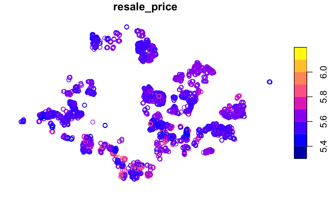

Although this is simply an initial visualisation of the dataset, it shows a brief idea of the spread of the sales across Singapore. There is a slight clustering near the central region indicating the prices are higher than the rest of the region. This is a useful indicator for variable selection.

3.2.6 Save Checkpoint as RDS file

Save file

write_rds(resale, "data/aspatial/rds/resale.rds")

Read File

resale <- read_rds("data/aspatial/rds/resale.rds")

3.3 Geospatial Data

The geospatial data used is the base map layer of Singapore and locational factors. For ease of use, the factors will be grouped by category (transport, education, sports, amenities and others).

Bus Stop
MRT

Kindergartens
Childcare
Primary Schools
Good Primary Schools

Sports Facilities
Parks
Gyms
Water Sites

Hawker Centers
Supermarkets
Eldercare

CBD Area
Waste Disposal
Active Cemeteries
Historic Sites

3.3.1 Load Data and Transform CRS

Store token for using onemap api

token <- "your token"

mpsz <- st_read(dsn = "data/geospatial/base", layer="MP14_SUBZONE_WEB_PL") %>%
  st_transform(crs = 3414)

Bus Stop

busstop <- st_read(dsn = "data/geospatial/transport/BusStop", layer="BusStop") %>%
  st_transform(crs = 3414) %>%
  select(1)

MRT

Code

#extract MRT data and save as shapefile
mrt <- st_read(dsn= "data/geospatial/transport/MRT/lta-mrt-station-exit-kml.kml") |> 
  st_zm()

st_write(obj = mrt,
         dsn = "data/geospatial/transport/MRT",
         layer = "MRT",
         driver = "ESRI Shapefile",
         append = FALSE)

#read shapefile
mrt <- st_read(dsn= "data/geospatial/transport/MRT", layer = "MRT") %>%
  st_transform(crs = 3414) %>%
  select(1)

Kindergartens

Code

#extract kindergarten data and save as shapefile
kindergartens<-get_theme(token,"kindergartens")
kindergartens <- st_as_sf(kindergartens, coords=c("Lng", "Lat"), crs=4326)

st_write(obj = kindergartens,
         dsn = "data/geospatial/education/kindergartens",
         layer = "kindergartens",
         driver = "ESRI Shapefile")

kindergartens <- st_read(dsn = "data/geospatial/education/kindergartens", layer = "kindergartens") %>%
  st_transform(crs = 3414) %>%
  select(1)

Childcare centers

Code

#extract childcare center data and save as shapefile
childcare<-get_theme(token,"childcare")
childcare <- st_as_sf(childcare, coords=c("Lng", "Lat"), crs=4326)

st_write(obj = childcare,
         dsn = "data/geospatial/education/childcare",
         layer = "childcare",
         driver = "ESRI Shapefile")

childcare <- st_read(dsn = "data/geospatial/education/childcare", layer = "childcare") %>%
  st_transform(crs = 3414) %>%
  select(1)

Primary school

Code

primary_schools <- read.csv("data/geospatial/education/primary_schools/general-information-of-schools.csv") |> 
  filter(mainlevel_code=="PRIMARY") |> 
  select(school_name, address, postal_code)


#dataframe to store api data
coords <- data.frame()

for (i in primary_schools$postal_code) {
  
  r <- GET('https://developers.onemap.sg/commonapi/search?',
           query=list(searchVal=i,
                     returnGeom='Y',
                     getAddrDetails='N'))
  
  data <- fromJSON(rawToChar(r$content))
  found <- data$found
  res <- data$results
  
  if (found > 0){
      lat <- res[[1]]$LATITUDE
      lng <- res[[1]]$LONGITUDE
      
      new_row <- data.frame(postal = as.numeric(i), latitude = lat, longitude = lng)
  }
  else {
    new_row <- data.frame(postal = as.numeric(i), latitude = NA, longitude = NA)
  }
  coords <- rbind(coords, new_row)
}

#There are 3 missing coordinate data for postal codes 88256, 99757 and 99840
#This is because the codes have 5 instead of 6 digits and need 0 padding

coords <- na.omit(coords)

for (i in c("088256", "099757", "099840")) {
  r <- GET('https://developers.onemap.sg/commonapi/search?',
           query=list(searchVal=i,
                     returnGeom='Y',
                     getAddrDetails='N'))
  
  res <- fromJSON(rawToChar(r$content))$results
  new_row <- data.frame(postal = as.numeric(i), latitude = res[[1]]$LATITUDE, longitude = res[[1]]$LONGITUDE)
  coords <- rbind(coords, new_row)
}


#add coordinate data into dataframe
primary_schools <- left_join(primary_schools, coords, by = c('postal_code' = 'postal'))

#store as sf object
primary_schools <- st_as_sf(primary_schools, coords=c("longitude", "latitude"), crs=4326)

#save as shapefile
st_write(obj = primary_schools,
         dsn = "data/geospatial/education/primary_schools",
         layer = "primary_schools",
         driver = "ESRI Shapefile")

primary_schools <- st_read(dsn = "data/geospatial/education/primary_schools", layer = "primary_schools") %>%
  st_transform(crs = 3414) %>%
  select(1)

Good primary school

The top 10 schools have been selected from here. Although this is 2020 data, it’s ranking structure was more holistic as it was not solely based on GEP.

Code

school_list <- toupper(c("Nanyang Primary School", "Tao Nan School", "Catholic High School", "Nan Hua Primary School", "St. Hilda's Primary School", "Henry Park Primary School", "Anglo-Chinese School (Primary)", "Raffles Girls' Primary School", "Pei Hwa Presbyterian Primary School", "Chij St. Nicholas Girls' School"))

good_primary_schools <- primary_schools %>%
  filter(schl_nm %in% school_list)


#There is a discrepency between the way Catholic High School and Chij St. Nicholas Girls' School are mentioned in the school list on the website but not in the list imported from onemap api. To simplify this, the next two best schools will be selected.

school_list <- toupper(c("Rosyth School", "Kong Hwa School"))

good_primary_schools <- rbind(good_primary_schools, primary_schools %>% filter(schl_nm %in% school_list))

#save as shapefile
st_write(obj = good_primary_schools,
         dsn = "data/geospatial/education/good_primary_schools",
         layer = "good_primary_schools",
         driver = "ESRI Shapefile")

good_primary_schools <- st_read(dsn = "data/geospatial/education/good_primary_schools", layer = "good_primary_schools") %>%
  st_transform(crs = 3414) %>%
  select(1)

Sports Facilities

Code

#extract sports facilities data and save as shapefile
sport_facilities <- get_theme(token,"sportsg_sport_facilities")

#Longitute column contains "longitute|latitude" which needs to be cleaned
sport_facilities <- sport_facilities %>%
  mutate(Lng=str_extract(Lng, "\\d+\\.?\\d*")) %>%
  select("NAME", "Lng", "Lat")

sport_facilities <- st_as_sf(sport_facilities, coords=c("Lng", "Lat"), crs=4326)

# creating a saved sf object in data file for easy reference
st_write(obj = sport_facilities,
         dsn = "data/geospatial/sports/sport_facilities",
         layer = "sport_facilities",
         driver = "ESRI Shapefile")

sport_facilities <- st_read(dsn = "data/geospatial/sports/sport_facilities", layer = "sport_facilities") %>%
  st_transform(crs = 3414) %>%
  select(1)

Parks

Code

#extract park data and save as shapefile
parks <- st_read(dsn= "data/geospatial/sports/parks/parks.kml") |> 
  st_zm()

st_write(obj = parks,
         dsn = "data/geospatial/sports/parks",
         layer = "parks",
         driver = "ESRI Shapefile",
         append = FALSE)

#read shapefile
parks <- st_read(dsn= "data/geospatial/sports/parks", layer = "parks") %>%
  st_transform(crs = 3414) %>%
  select(1)

Gyms

Code

#extract gym data and save as shapefile
gyms <- st_read(dsn= "data/geospatial/sports/gyms/gyms-sg-kml.kml") |> 
  st_zm()

st_write(obj = gyms,
         dsn = "data/geospatial/sports/gyms",
         layer = "gyms",
         driver = "ESRI Shapefile",
         append = FALSE)

#read shapefile
gyms <- st_read(dsn= "data/geospatial/sports/gyms", layer = "gyms") %>%
  st_transform(crs = 3414) %>%
  select(1)

Water Sites

Code

#extract gym data and save as shapefile
watersites <- st_read(dsn= "data/geospatial/sports/watersites/abc-water-sites.kml") |> 
  st_zm()

st_write(obj = watersites,
         dsn = "data/geospatial/sports/watersites",
         layer = "watersites",
         driver = "ESRI Shapefile",
         append = FALSE)

#read shapefile
watersites <- st_read(dsn= "data/geospatial/sports/watersites", layer = "watersites") %>%
  st_transform(crs = 3414) %>%
  select(1)

Hawker centers

Code

#extract gym data and save as shapefile
hawker_centers <- st_read(dsn= "data/geospatial/amenities/hawker_centers/hawker-centres-kml.kml") |> 
  st_zm()

st_write(obj = hawker_centers,
         dsn = "data/geospatial/amenities/hawker_centers",
         layer = "hawker_centers",
         driver = "ESRI Shapefile",
         append = FALSE)

#read shapefile
hawker_centers <- st_read(dsn= "data/geospatial/amenities/hawker_centers", layer = "hawker_centers") %>%
  st_transform(crs = 3414) %>%
  select(1)

Supermarkets

Code

#extract gym data and save as shapefile
supermarkets <- st_read(dsn= "data/geospatial/amenities/supermarkets/supermarkets-kml.kml") |> 
  st_zm()

st_write(obj = supermarkets,
         dsn = "data/geospatial/amenities/supermarkets",
         layer = "supermarkets",
         driver = "ESRI Shapefile",
         append = FALSE)

#read shapefile
supermarkets <- st_read(dsn= "data/geospatial/amenities/supermarkets", layer = "supermarkets") %>%
  st_transform(crs = 3414) %>%
  select(1)

Eldercare

Code

#extract eldercare center data and save as shapefile
eldercare <-get_theme(token,"eldercare")
eldercare <- st_as_sf(eldercare, coords=c("Lng", "Lat"), crs=4326)

st_write(obj = eldercare,
         dsn = "data/geospatial/amenities/eldercare",
         layer = "eldercare",
         driver = "ESRI Shapefile")

eldercare <- st_read(dsn = "data/geospatial/amenities/eldercare", layer = "eldercare") %>%
  st_transform(crs = 3414) %>%
  select(1)

CBD Area

As the ‘Downtown Core’ is also referred to as the Central Business District (CBD), the coordinates of ‘Downtown Core’ shall be used. Based on the information here, the latitude is 1.287953 and longitude is 103.851784

cbd <- st_as_sf(data.frame(name = c("CBD Area"), latitude = c(1.287953), longitude = c(103.851784)),
                coords = c("longitude", "latitude"),
                crs = 3414)

Waste Disposal sites

Code

#extract waste disposal data and save as shapefile
waste_disposal <- st_read(dsn= "data/geospatial/others/waste_disposal/waste-treatment-kml.kml") |> 
  st_zm()

st_write(obj = supermarkets,
         dsn = "data/geospatial/others/waste_disposal",
         layer = "waste_disposal",
         driver = "ESRI Shapefile",
         append = FALSE)

#read shapefile
waste_disposal <- st_read(dsn= "data/geospatial/others/waste_disposal", layer = "waste_disposal") %>%
  st_transform(crs = 3414) %>%
  select(1)

Active Cemeteries

Code

#extract active cemeteries data and save as shapefile
cemeteries <- st_read(dsn= "data/geospatial/others/active_cemeteries/active-cemeteries-kml.kml") |> 
  st_zm()

st_write(obj = cemeteries,
         dsn = "data/geospatial/others/active_cemeteries",
         layer = "cemeteries",
         driver = "ESRI Shapefile",
         append = FALSE)

#read shapefile
cemeteries <- st_read(dsn= "data/geospatial/others/active_cemeteries", layer = "cemeteries") %>%
  st_transform(crs = 3414) %>%
  select(1)

Historic Sites

Code

#extract historic sites data and save as shapefile
historic_sites <- st_read(dsn= "data/geospatial/others/historic_sites/historic-sites-kml.kml") |> 
  st_zm()

st_write(obj = historic_sites,
         dsn = "data/geospatial/others/historic_sites",
         layer = "historic_sites",
         driver = "ESRI Shapefile",
         append = FALSE)

#read shapefile
historic_sites <- st_read(dsn= "data/geospatial/others/historic_sites", layer = "historic_sites") %>%
  st_transform(crs = 3414) %>%
  select(1)

3.3.2 Check for Invalid Geometries

3.3.2.1 Base layer

Code

c <- 9 #length(which(st_is_valid(mpsz) == FALSE))
cat("There are", c , "invalid geometries in the base layer. This shall be resolved in the following step.")

There are 9 invalid geometries in the base layer. This shall be resolved in the following step.

mpsz <- st_make_valid(mpsz)

Code

c <- 0 #length(which(st_is_valid(mpsz) == FALSE))
cat("There are now", c , "invalid geometries in the base layer.")

There are now 0 invalid geometries in the base layer.

3.3.2.2 Geospatial Factors

Code

df_list <- c("busstop", "cbd", "cemeteries", "childcare", "eldercare", "good_primary_schools", "gyms", "hawker_centers", "historic_sites", "kindergartens", "mrt", "parks", "primary_schools", "sport_facilities", "supermarkets", "waste_disposal", "watersites")

c = 0 
for(i in df_list) {
  c = c + length(which(st_is_valid(eval(parse(text = i))) == FALSE))
}

Code

c = 0 
cat("There are", c , "invalid geometries in the geospatial factors")

There are 0 invalid geometries in the geospatial factors

3.3.3 Check for Missing Values

3.3.3.1 Base layer

Code

c = 0 #sum(is.na(mpsz))
cat("There are", c , "missing values in the base layer.")

There are 0 missing values in the base layer.

3.3.3.2 Geospatial Factors

Code

c = 0 
for(i in df_list) {
  c = c + sum(is.na(mpsz))
}

Code

c = 0
cat("There are", c , "missing values in the geospatial factors.")

There are 0 missing values in the geospatial factors.

3.3.4 Verify CRS

3.3.4.1 Base layer

st_crs(mpsz)[1]$input

3.3.4.2 Geospatial Factors

Code

for(i in df_list) {
  cat(i, st_crs(eval(parse(text = i)))[1]$input, "\n")
}

3.4 Visualise Data

Code

tm_shape(mpsz) +
  tm_borders(alpha = 0.5) +
  tmap_options(check.and.fix = TRUE) +
tm_shape(busstop) +
  tm_dots(col="azure3", alpha=0.5) +
tm_shape(mrt) +
  tm_dots(col="yellow", alpha=1)+
  tm_layout(main.title = "Transport",
          main.title.position = "center")

Code

tm_shape(mpsz) +
  tm_borders(alpha = 0.5) +
  tmap_options(check.and.fix = TRUE) +
tm_shape(childcare) +
  tm_dots(col="black", alpha=0.2) +
tm_shape(primary_schools) +
  tm_dots(col="lightskyblue3", alpha=0.5)+
tm_shape(kindergartens) +
  tm_dots(col="lightslateblue", alpha=0.5) +
tm_shape(good_primary_schools) +
  tm_dots(col="red", alpha=1)+
tm_shape(mpsz) +
  tm_borders(alpha = 0.01) +
  tm_layout(main.title = "Education",
          main.title.position = "center")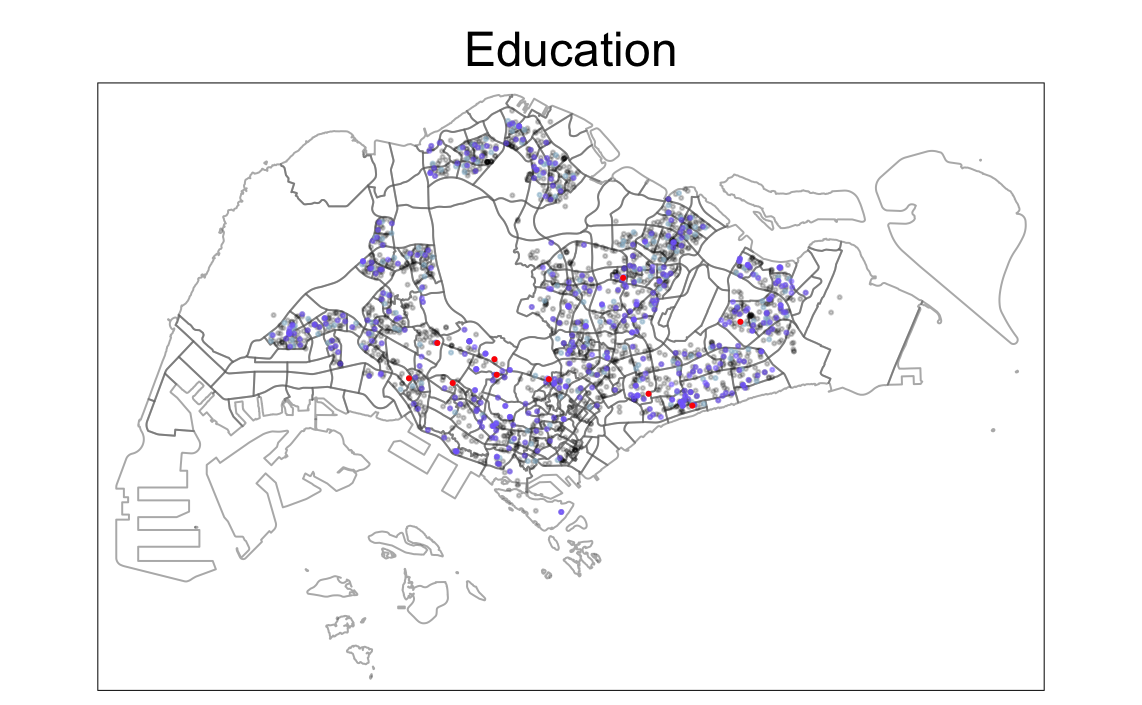

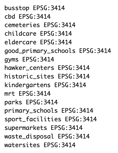
Code

tm_shape(mpsz) +
  tm_borders(alpha = 0.5) +
  tmap_options(check.and.fix = TRUE) +
tm_shape(sport_facilities) +
  tm_dots(col="violet", alpha=1) +
tm_shape(parks) +
  tm_dots(col="mediumseagreen", alpha=0.5) + 
tm_shape(gyms) +
  tm_dots(col="azure3", alpha=0.7) +
tm_shape(watersites) +
  tm_dots(col="skyblue3", alpha=1) +
  tm_layout(main.title = "Sports",
          main.title.position = "center")

Code

tm_shape(mpsz) +
  tm_borders(alpha = 0.5) +
  tmap_options(check.and.fix = TRUE) +
tm_shape(hawker_centers) +
  tm_dots(col="firebrick3", alpha=1) +
tm_shape(supermarkets) +
  tm_dots(col="olivedrab", alpha=0.5) + 
tm_shape(eldercare) +
  tm_dots(col="tan", alpha=0.7) +
  tm_layout(main.title = "Amenities",
          main.title.position = "center")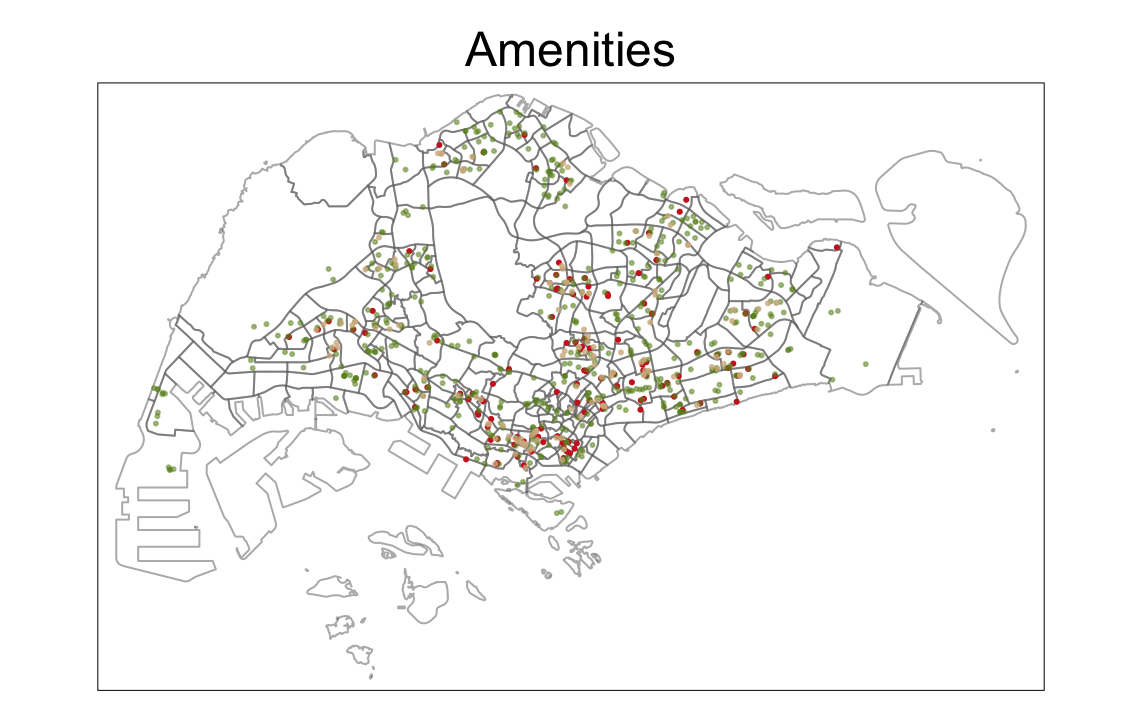

Code

tm_shape(mpsz) +
  tm_borders(alpha = 0.5) +
  tmap_options(check.and.fix = TRUE) +
tm_shape(cbd) +
  tm_dots(col="purple", alpha=1) +
tm_shape(waste_disposal) +
  tm_dots(col="coral3", alpha=0.5) + 
tm_shape(cemeteries) +
  tm_dots(col="gray20", alpha=1) +
tm_shape(historic_sites) +
  tm_dots(col="darkseagreen2", alpha=1) +
  tm_layout(main.title = "Others",
          main.title.position = "center")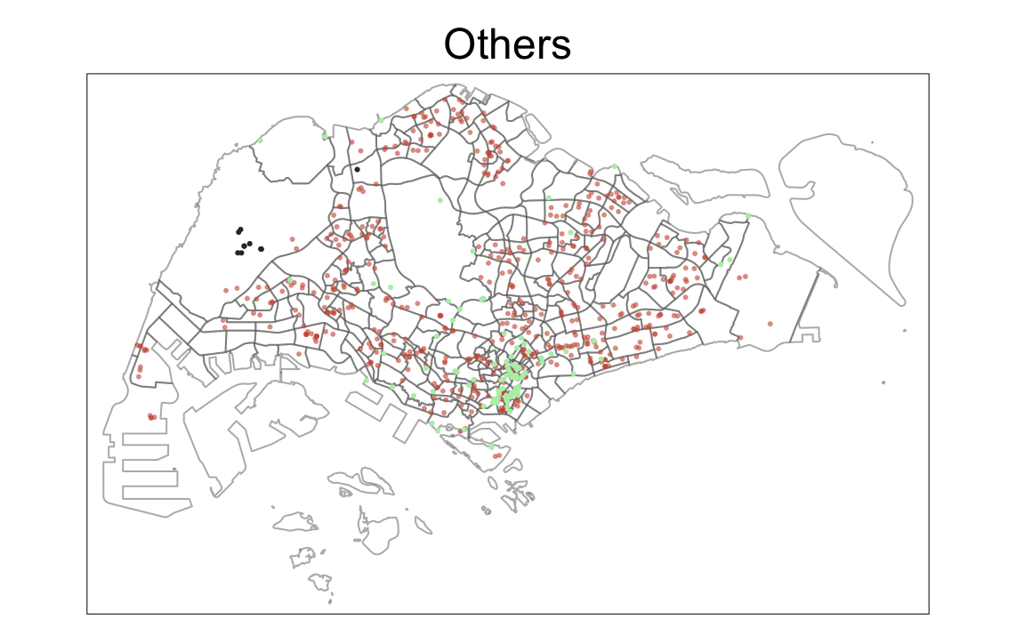

4.0 Regression Modelling

4.1 Proximity Calculation

for(i in df_list) {
  dist_matrix <- st_distance(resale, eval(parse(text = i))) |> drop_units()
  resale[,paste("PROX_",toupper(i), sep = "")] <- rowMins(dist_matrix)
}

4.2 Count in range Calculation

num_list <- c("kindergartens", "childcare", "busstop", "primary_schools")
radius_list <- c(350, 350, 350, 1000)
for(i in 1:4) {
  dist_matrix <- st_distance(resale, eval(parse(text = num_list[i]))) |> drop_units()
  resale[,paste("NUM_",toupper(num_list[i]),"_WITHIN_",radius_list[i],"M", sep = "")] <- rowSums(dist_matrix <= radius_list[i])
}

4.3 Save checkpoint as RDS file

Save file

write_rds(resale, "data/rds/resale.rds")

Read file

Code

df_list <- c("busstop", "cbd", "cemeteries", "childcare", "eldercare", "good_primary_schools", "gyms", "hawker_centers", "historic_sites", "kindergartens", "mrt", "parks", "primary_schools", "sport_facilities", "supermarkets", "waste_disposal", "watersites")
prox <- paste("PROX_",toupper(df_list), sep="")
others <- c("floor_area_sqm", "remaining_lease", "storey_num", "NUM_KINDERGARTENS_WITHIN_350M", "NUM_CHILDCARE_WITHIN_350M", "NUM_BUSSTOP_WITHIN_350M", "NUM_PRIMARY_SCHOOLS_WITHIN_1000M", "resale_price", "month")
df_list <- c(prox, others)

resale <- read_rds("data/rds/resale.rds") %>%
  select(df_list)

4.4 Data Preparation

4.4.1 Correlation Matrix

To check for multicolinearity

Code

corr <- resale |>
  select_if(is.numeric) |>
  st_drop_geometry() |>
  select(-resale_price)

corrplot(cor(corr),
         diag = FALSE,
         order = "AOE",
         tl.pos = "td",
         tl.cex = 0.5,
         method = "number",
           type = "upper")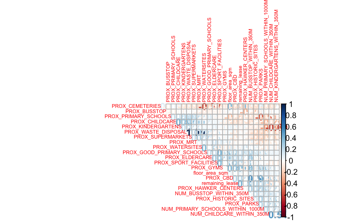

Variables are not correlated to each other so all values can be selected for the model

4.4.2 Data Sampling

Seperate data into train and test. Train data - all transactions between Jan 01 2021 to Dec 31 2021. Test data - Jan 01 2023 to Feb 28 2023

train_data<-resale |>
  filter(month >= "2021-01" & month <= "2022-12") |>
  select(-c(month))

test_data<-resale |>
  filter(month >= "2023-01" & month <= "2023-02") |>
  select(-c(month))

4.4.2.1 Save Train and Test data as Checkpoint

Save file

write_rds(train_data, "data/rds/train_data.rds")
write_rds(test_data, "data/rds/test_data.rds")

Read file

train_data <- read_rds("data/rds/train_data.rds")
test_data <- read_rds("data/rds/test_data.rds")

4.5 OLS method

Non Spatial Multiple Linear Regression using OLS method

4.5.1 Train model

Code

mlr<- lm(resale_price ~ floor_area_sqm + remaining_lease + storey_num + PROX_BUSSTOP + PROX_CBD + PROX_CEMETERIES + PROX_CHILDCARE + PROX_ELDERCARE + PROX_GOOD_PRIMARY_SCHOOLS + PROX_GYMS + PROX_HAWKER_CENTERS + PROX_HISTORIC_SITES + PROX_KINDERGARTENS + PROX_MRT + PROX_PARKS + PROX_PRIMARY_SCHOOLS + PROX_SPORT_FACILITIES + PROX_SUPERMARKETS + PROX_WASTE_DISPOSAL + PROX_WATERSITES + NUM_KINDERGARTENS_WITHIN_350M + NUM_CHILDCARE_WITHIN_350M + NUM_BUSSTOP_WITHIN_350M + NUM_PRIMARY_SCHOOLS_WITHIN_1000M,
         data = train_data)

# save result
write_rds(mlr, "data/rds/mlr.rds")

Summary

mlr<-read_rds("data/rds/mlr.rds")
ols_regress(mlr)

                        Model Summary                         
-------------------------------------------------------------
R                       0.785       RMSE               0.056 
R-Squared               0.617       Coef. Var          1.004 
Adj. R-Squared          0.616       MSE                0.003 
Pred R-Squared          0.615       MAE                0.044 
-------------------------------------------------------------
 RMSE: Root Mean Square Error 
 MSE: Mean Square Error 
 MAE: Mean Absolute Error 

                                 ANOVA                                  
-----------------------------------------------------------------------
               Sum of                                                  
              Squares           DF    Mean Square       F         Sig. 
-----------------------------------------------------------------------
Regression     63.111           21          3.005    964.682    0.0000 
Residual       39.209        12586          0.003                      
Total         102.320        12607                                     
-----------------------------------------------------------------------

                                            Parameter Estimates                                             
-----------------------------------------------------------------------------------------------------------
                        model      Beta    Std. Error    Std. Beta       t        Sig      lower     upper 
-----------------------------------------------------------------------------------------------------------
                  (Intercept)     5.147         0.008                 661.132    0.000     5.131     5.162 
               floor_area_sqm     0.005         0.000        0.352     62.173    0.000     0.005     0.005 
              remaining_lease     0.004         0.000        0.777    114.321    0.000     0.004     0.004 
                 PROX_BUSSTOP     0.000         0.000       -0.005     -0.880    0.379     0.000     0.000 
                     PROX_CBD     0.000         0.000       -0.313    -32.586    0.000     0.000     0.000 
              PROX_CEMETERIES     0.000         0.000        0.362     37.583    0.000     0.000     0.000 
               PROX_CHILDCARE     0.000         0.000       -0.015     -2.180    0.029     0.000     0.000 
               PROX_ELDERCARE     0.000         0.000       -0.012     -1.892    0.059     0.000     0.000 
    PROX_GOOD_PRIMARY_SCHOOLS     0.000         0.000        0.046      4.995    0.000     0.000     0.000 
                    PROX_GYMS     0.000         0.000       -0.071     -8.914    0.000     0.000     0.000 
          PROX_HAWKER_CENTERS     0.000         0.000       -0.063     -9.556    0.000     0.000     0.000 
          PROX_HISTORIC_SITES     0.000         0.000       -0.059     -7.781    0.000     0.000     0.000 
           PROX_KINDERGARTENS     0.000         0.000       -0.014     -1.727    0.084     0.000     0.000 
                     PROX_MRT     0.000         0.000       -0.100    -16.453    0.000     0.000     0.000 
                   PROX_PARKS     0.000         0.000       -0.092    -14.879    0.000     0.000     0.000 
         PROX_PRIMARY_SCHOOLS     0.000         0.000       -0.010     -1.562    0.118     0.000     0.000 
        PROX_SPORT_FACILITIES     0.000         0.000        0.019      2.813    0.005     0.000     0.000 
            PROX_SUPERMARKETS     0.000         0.000        0.032      4.917    0.000     0.000     0.000 
          PROX_WASTE_DISPOSAL        NA         0.000       -0.007     -3.894    0.000        NA        NA 
              PROX_WATERSITES     0.000         0.001       30.955      4.484    0.000     0.000     0.000 
NUM_KINDERGARTENS_WITHIN_350M     0.004         0.000       -0.014     -4.556    0.000     0.002     0.005 
    NUM_CHILDCARE_WITHIN_350M    -0.001         0.000        0.018      3.808    0.000    -0.002    -0.001 
      NUM_BUSSTOP_WITHIN_350M     0.001            NA        0.144         NA       NA     0.000     0.001 
-----------------------------------------------------------------------------------------------------------

With a final adjusted R squared of 61.6%, the model does show scope for imporvement especially in terms of reducing cardinality by removing variables like proximity to waste disposal sites and other variables with low significance (p value < 0.05)

4.5.2 Check Model

ols_vif_tol(mlr)

                       Variables Tolerance      VIF
1                 floor_area_sqm 0.9490861 1.053645
2                remaining_lease 0.6588448 1.517808
3                   PROX_BUSSTOP 0.8923011 1.120698
4                       PROX_CBD 0.3297989 3.032151
5                PROX_CEMETERIES 0.3286168 3.043058
6                 PROX_CHILDCARE 0.6451561 1.550012
7                 PROX_ELDERCARE 0.7112568 1.405962
8      PROX_GOOD_PRIMARY_SCHOOLS 0.3515867 2.844249
9                      PROX_GYMS 0.4798414 2.084022
10           PROX_HAWKER_CENTERS 0.7096034 1.409238
11           PROX_HISTORIC_SITES 0.5239897 1.908434
12            PROX_KINDERGARTENS 0.4778528 2.092695
13                      PROX_MRT 0.8318112 1.202196
14                    PROX_PARKS 0.7960906 1.256138
15          PROX_PRIMARY_SCHOOLS 0.7762761 1.288201
16         PROX_SPORT_FACILITIES 0.6764521 1.478301
17             PROX_SUPERMARKETS 0.0000000      Inf
18           PROX_WASTE_DISPOSAL 0.0000000      Inf
19               PROX_WATERSITES 0.6337165 1.577993
20 NUM_KINDERGARTENS_WITHIN_350M 0.4660639 2.145629
21     NUM_CHILDCARE_WITHIN_350M 0.6068474 1.647861
22       NUM_BUSSTOP_WITHIN_350M 0.8183733 1.221936

All values are less than 10 which means the variables are not multicolinear.

ols_plot_resid_fit(mlr)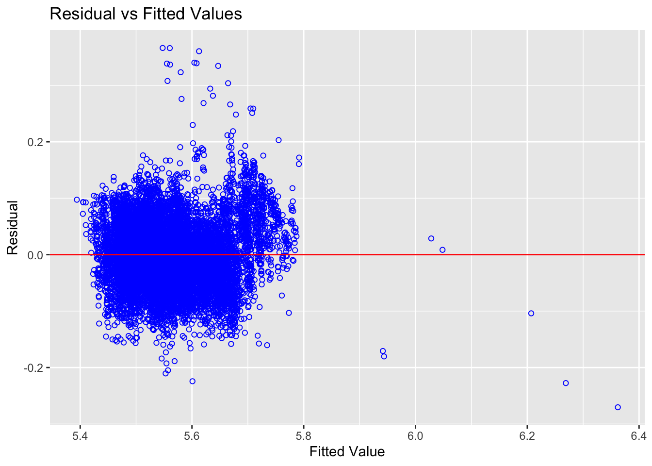

As most of the variables are scattered around the 0 line, the relationships between the dependent variable and independent variables are linear.

ols_plot_resid_hist(mlr)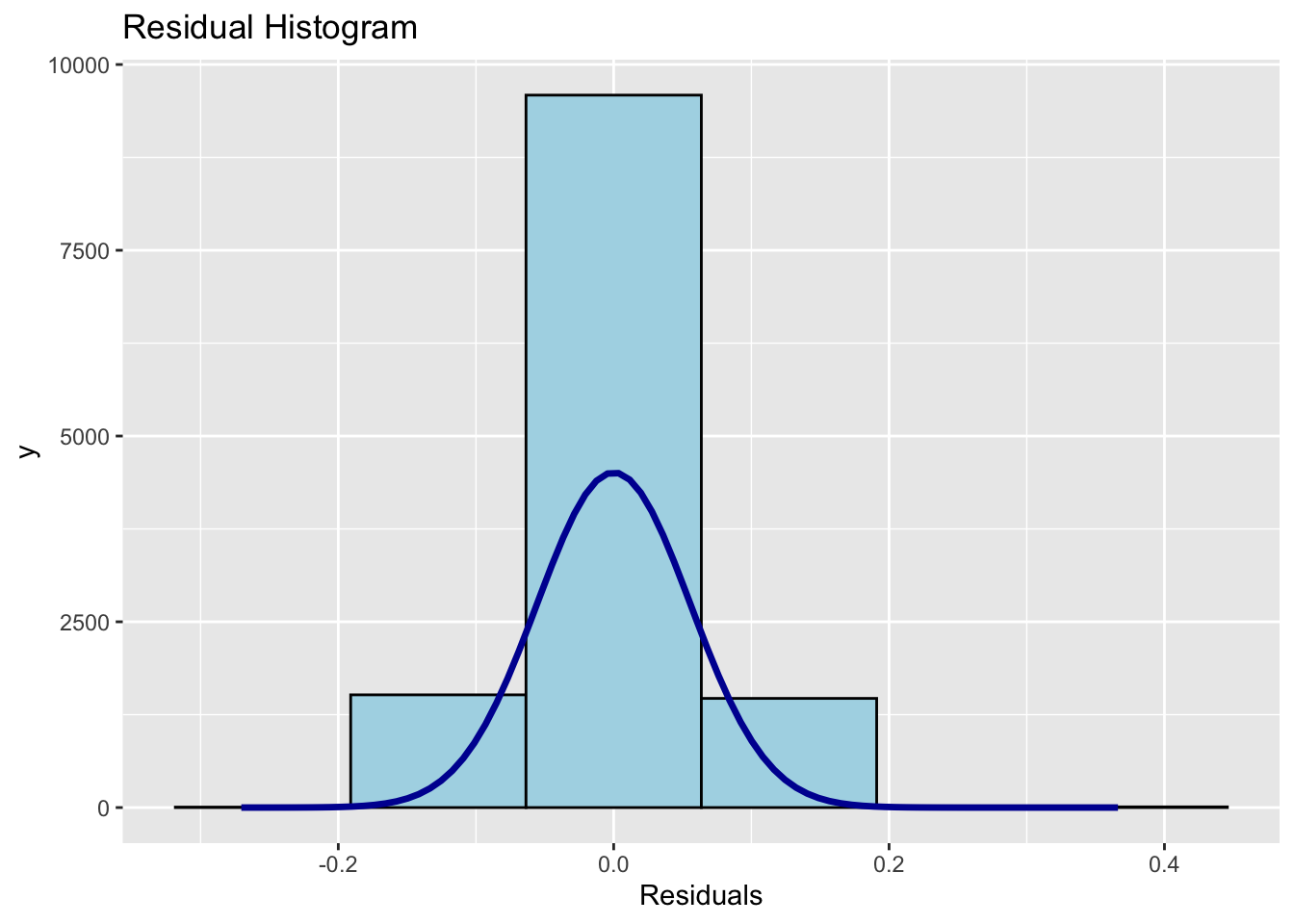

Normal distribution is followed

4.5.3 Test Model

4.5.3.1 Generate Predictions

mlr_pred <- as.data.frame(predict(mlr, 
                    newdata = test_data, 
                    interval = 'confidence'))

#Store as RDS
test_data_mlr <- cbind(test_data, mlr_pred)
write_rds(test_data_mlr, "data/rds/test_data_mlr.rds")

4.5.3.2 Root Mean Square Error (RSME)

Code

test_data_mlr <- read_rds("data/rds/test_data_mlr.rds")
rmse(test_data_mlr$resale_price, test_data_mlr$fit)

[1] 0.06123716

As the value is less than 0.1, it means the model is able to satisfactory predictions.

4.5.3.3 Visualise

Actual vs. predicted values

ggplot(data = test_data_mlr,
       aes(x = fit, y = resale_price)) +
  geom_point()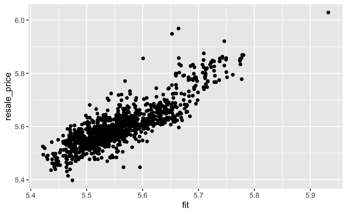

4.6 GWR predictive method

4.6.1 Convert to spatial points dataframe

train_data.sp <- as_Spatial(train_data)

4.6.2 Compute adaptive bandwidth

Code

adaptive_bw <- bw.gwr(resale_price ~ floor_area_sqm + remaining_lease + storey_num + PROX_BUSSTOP + PROX_CBD + PROX_CEMETERIES + PROX_CHILDCARE + PROX_ELDERCARE + PROX_GOOD_PRIMARY_SCHOOLS + PROX_GYMS + PROX_HAWKER_CENTERS + PROX_HISTORIC_SITES + PROX_KINDERGARTENS + PROX_MRT + PROX_PARKS + PROX_PRIMARY_SCHOOLS + PROX_SPORT_FACILITIES + PROX_SUPERMARKETS + PROX_WASTE_DISPOSAL + PROX_WATERSITES + NUM_KINDERGARTENS_WITHIN_350M + NUM_CHILDCARE_WITHIN_350M + NUM_BUSSTOP_WITHIN_350M + NUM_PRIMARY_SCHOOLS_WITHIN_1000M,
                data=train_data.sp,
                approach="CV",
                kernel="gaussian",
                adaptive=TRUE,
                longlat=FALSE)
write_rds(adaptive_bw, "data/rds/adaptive_bw.rds")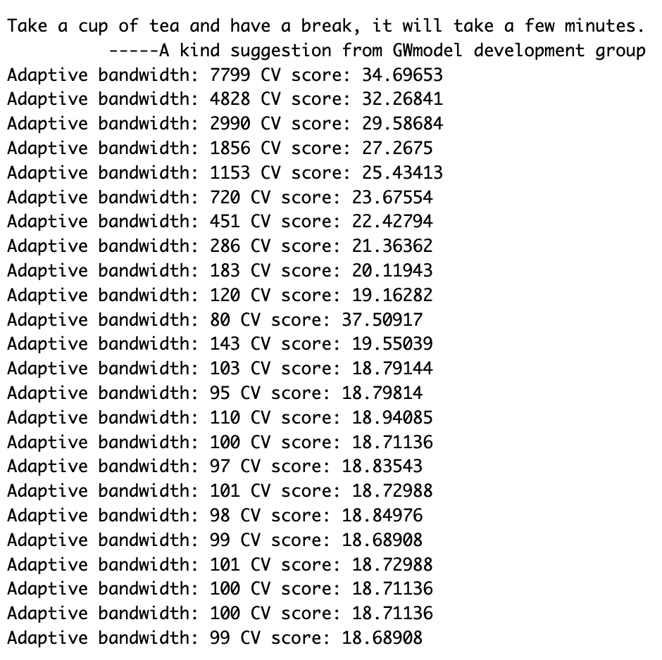

The output seems to have reached a local minima of 99m for the bandwidth.

4.6.3 Construct Model

Code

#read data
adaptive_bw <- read_rds("data/rds/adaptive_bw.rds")

#construct model
gwr_adaptive <- gwr.basic(formula = resale_price ~ floor_area_sqm + storey_num + remaining_lease + PROX_BUSSTOP + PROX_CBD + PROX_CEMETERIES + PROX_CHILDCARE + PROX_ELDERCARE + PROX_GOOD_PRIMARY_SCHOOLS + PROX_GYMS + PROX_HAWKER_CENTERS + PROX_HISTORIC_SITES + PROX_KINDERGARTENS + PROX_MRT + PROX_PARKS + PROX_SUPERMARKETS + PROX_PRIMARY_SCHOOLS + PROX_SPORT_FACILITIES + PROX_WASTE_DISPOSAL + PROX_WATERSITES + NUM_KINDERGARTENS_WITHIN_350M + NUM_CHILDCARE_WITHIN_350M + NUM_BUSSTOP_WITHIN_350M + NUM_PRIMARY_SCHOOLS_WITHIN_1000M,
                data=train_data.sp,
                bw = adaptive_bw,
                kernel="gaussian",
                adaptive=TRUE,
                longlat=FALSE)

#store data
write_rds(gwr_adaptive, "data/model/gwr_adaptive.rds")

4.6.3 Prepare Coordinates Data

4.6.3.1 Extract Coordinates

coords <- st_coordinates(resale)
coords_train <- st_coordinates(train_data)
coords_test <- st_coordinates(test_data)

Save as RDS file

coords_train <- write_rds(coords_train, "data/rds/coords_train.rds" )
coords_test <- write_rds(coords_test, "data/rds/coords_test.rds" )

4.6.3.2 Drop Geometry

train_data <- train_data %>% 
  st_drop_geometry()

4.7 Calibrate Random Forest Model

4.7.1 Compute adaptive bandwidth

Code

adaptive_bw <- grf.bw(formula = resale_price ~ floor_area_sqm + remaining_lease + PROX_BUSSTOP + PROX_CBD + PROX_CEMETERIES + PROX_CHILDCARE + PROX_ELDERCARE + PROX_GOOD_PRIMARY_SCHOOLS + PROX_GYMS + PROX_HAWKER_CENTERS + PROX_HISTORIC_SITES + PROX_KINDERGARTENS + PROX_MRT + PROX_PARKS + PROX_PRIMARY_SCHOOLS + PROX_SPORT_FACILITIES + PROX_WASTE_DISPOSAL + PROX_WATERSITES + NUM_KINDERGARTENS_WITHIN_350M + NUM_CHILDCARE_WITHIN_350M + NUM_BUSSTOP_WITHIN_350M + NUM_PRIMARY_SCHOOLS_WITHIN_1000M,
                data=train_data,
                kernel="adaptive",
                trees = 50,
                coords=coords_train)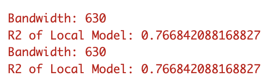

The bandwidth should be 630m

4.7.2 Generate model

Code

set.seed(1234)
gwRF_adaptive<-grf(formula = resale_price ~ floor_area_sqm + remaining_lease + storey_num + PROX_BUSSTOP + PROX_CBD + PROX_CEMETERIES + PROX_CHILDCARE + PROX_ELDERCARE + PROX_GOOD_PRIMARY_SCHOOLS + PROX_GYMS + PROX_SUPERMARKETS + PROX_HAWKER_CENTERS + PROX_HISTORIC_SITES + PROX_KINDERGARTENS + PROX_MRT + PROX_PARKS + PROX_PRIMARY_SCHOOLS + PROX_SPORT_FACILITIES + PROX_WASTE_DISPOSAL + PROX_WATERSITES + NUM_KINDERGARTENS_WITHIN_350M + NUM_CHILDCARE_WITHIN_350M + NUM_BUSSTOP_WITHIN_350M + NUM_PRIMARY_SCHOOLS_WITHIN_1000M,
                   dframe=train_data,
                   bw=630,
                   kernel="adaptive",
                   coords=coords_train,
                   ntree=50)

#save as rds
write_rds(gwRF_adaptive, "data/model/gwRF_adaptive.rds")

gwRF_adaptive$Global.Model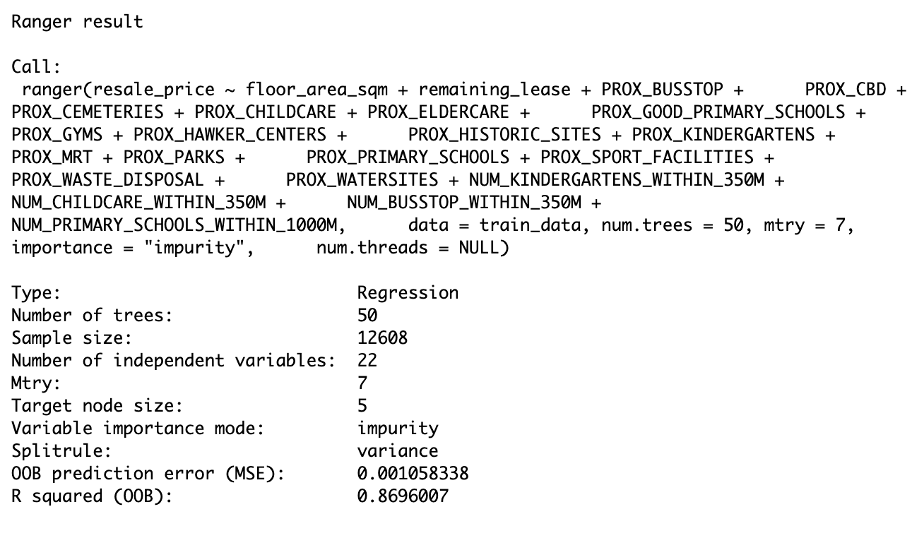

4.7.3 Test model

4.7.3.1 Prepare Test Data

test_data <- cbind(test_data, coords_test) %>%
  st_drop_geometry()

4.7.3.2 Generate Predictions

Code

gwRF_pred <- as.data.frame(predict.grf(gwRF_adaptive,
                           test_data,
                           x.var.name="X",
                           y.var.name="Y",
                           local.w=1,
                           global.w=0))

#Store as RDS
test_data_gwr <- cbind(test_data, gwRF_pred)
test_data_gwr <- test_data_gwr %>%
  rename(GRF_pred = `predict.grf(gwRF_adaptive, test_data, x.var.name = "X", y.var.name = "Y", local.w = 1, global.w = 0)`)

write_rds(gwRF_pred, "data/rds/GRF_pred.rds")

4.7.3.3 Root mean square error (RMSE)

Code

test_data_gwr <- read_rds("data/rds/GRF_pred.rds")
rmse(test_data$resale_price, test_data_gwr$GRF_pred)

[1] NaN

As the value is less than 0.1, it means the model is able to satisfactory predictions.

4.7.3.4 Visualise

Actual vs. predicted values

Code

ggplot(data = temp,
       aes(x = GRF_pred,
           y = resale_price)) +
  geom_point()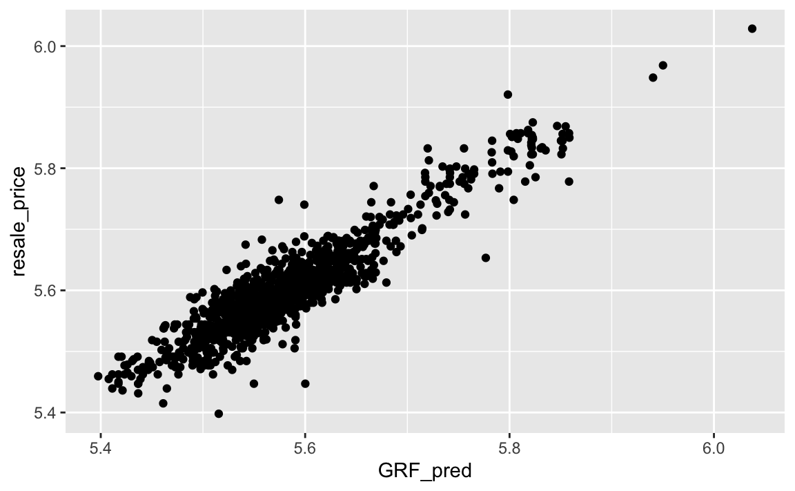

4.8 Comparison

Based on the root mean square error (RMSE) of the two models, the GWR model has a lower error of 0.03629414 whereas the OLS model had an error of 0.06123716. Although the difference is not that great, there are some reasons why they both performed well and why GWR method is more suitable.

Furthermore, based on the graphs, below, the GWR model seems to be more centered with a lower R squared than the OLS model.

OLS model
GWR model

Due to high cardinality of the data, both models ended up having similar performance. However, the OLS model makes several assumptions of normality and linearity. GWR on the other hand is more dynamic as is allows for spatial data to come and considers the local neighbourhood around each observation.

5.0 Acknowledgements

I’d like to thank Professor Kam for his insights and resource materials provided under IS415 Geospatial Analytics and Applications.